Installing R & RStudio vs. RStudio Cloud
If you want to use your own machine (not recommended except for the texh-savvy)
(1) First install the latest version of  from here
(2) Then install the latest version of  from here
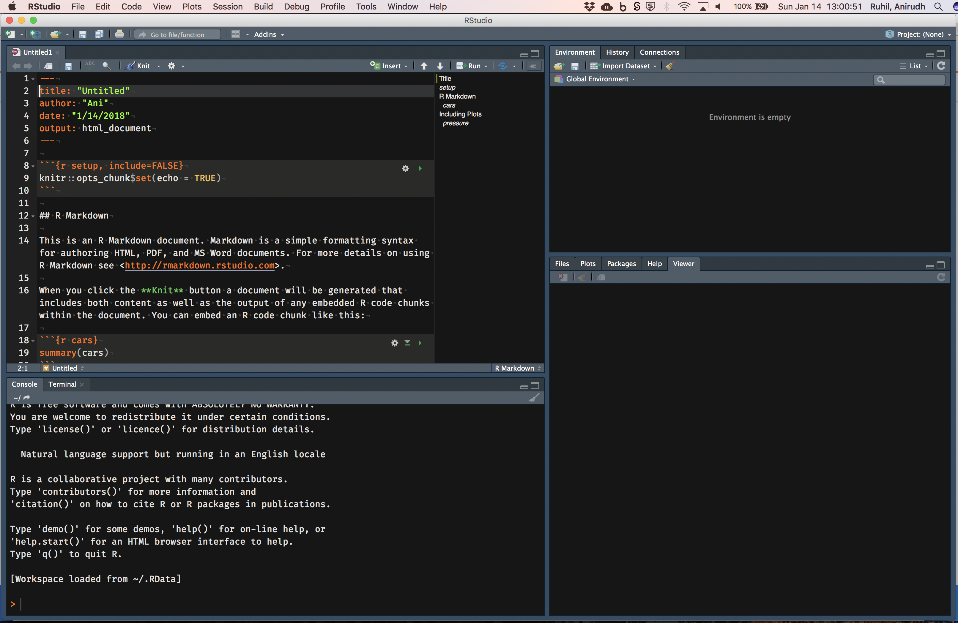
(3) Launch RStudio and check that it shows something like the image below:
Using Rstudio Cloud (recommended)
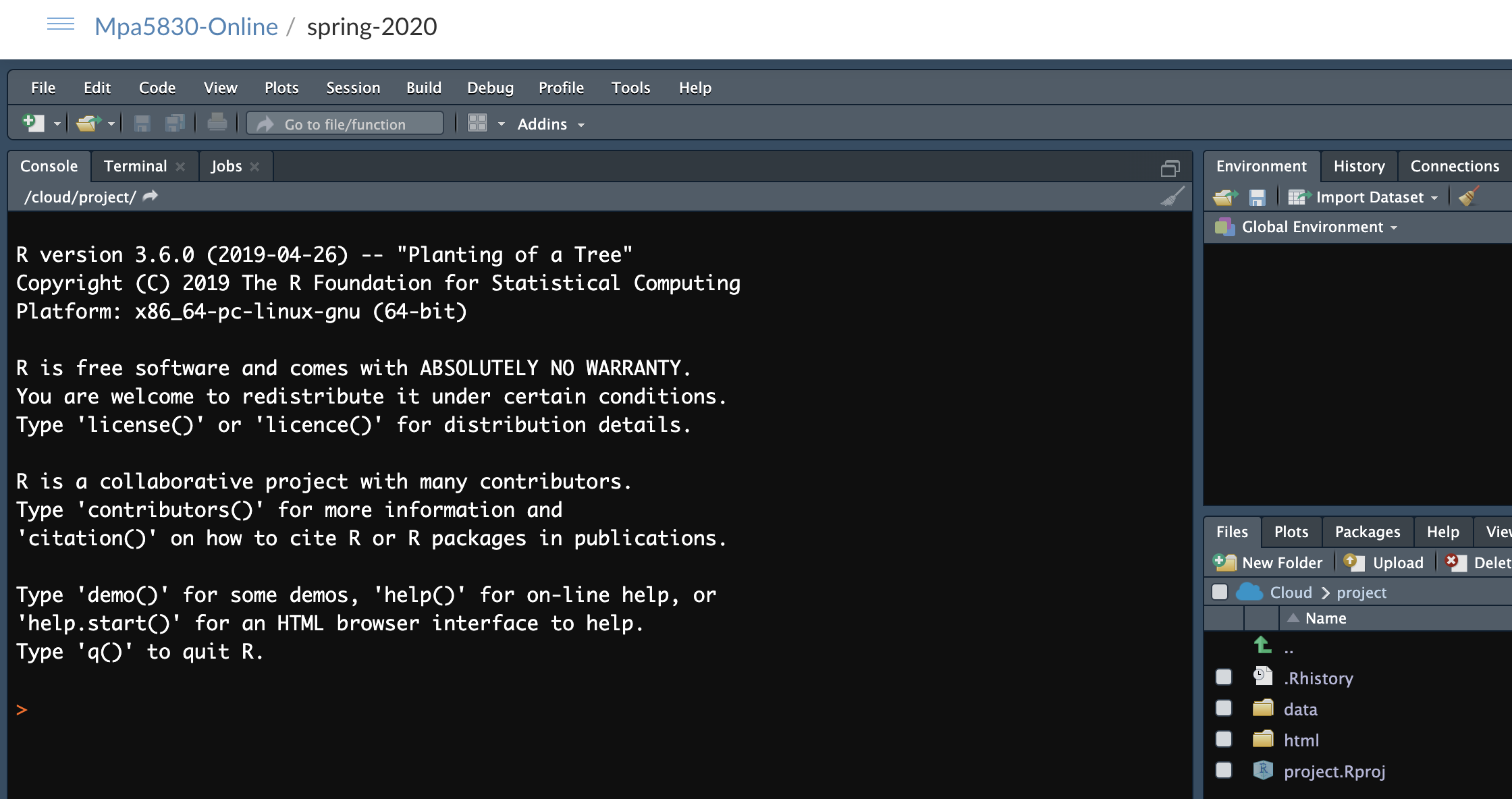
(1) Use the link you received in your email to create a free account on RStudio Cloud, and then to access the course project. Once you are logged into RStudio Cloud you should see a tab called "Project." Clicking on this should give you the following browser screen:
Understand your RStudio Environment
Rprojects (ONLY if installing on your own computer)
- Create a folder called mpa5830. Inside mpa5830 create ONE sub-folder called data. The folder structure will now be
mpa5830/ └── data/ └── datafile-1 └── datafile-2 └── ...- Create a
projectviaFile -> New Project, chooseExisting Directory,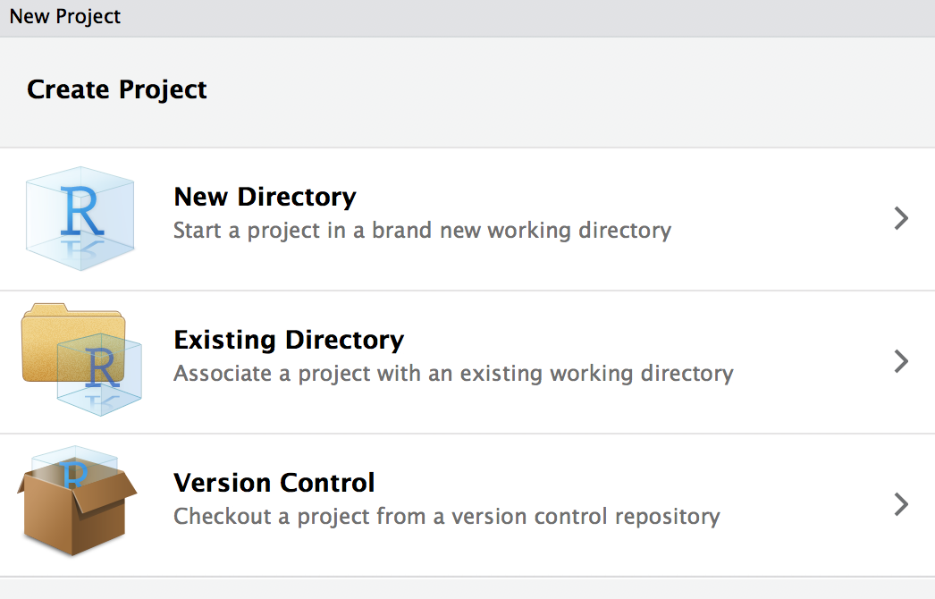
Browse to the mpa5830 folder
RStudio will restart and you will be in the project folder, seeing a file called
mpa5830.RprojFrom now on, start every session by double-clicking
mpa5830.Rproj
R Markdown files
- Go to
New File -> R Markdown ...and enter aMy First Rmd Filein title and yourname.
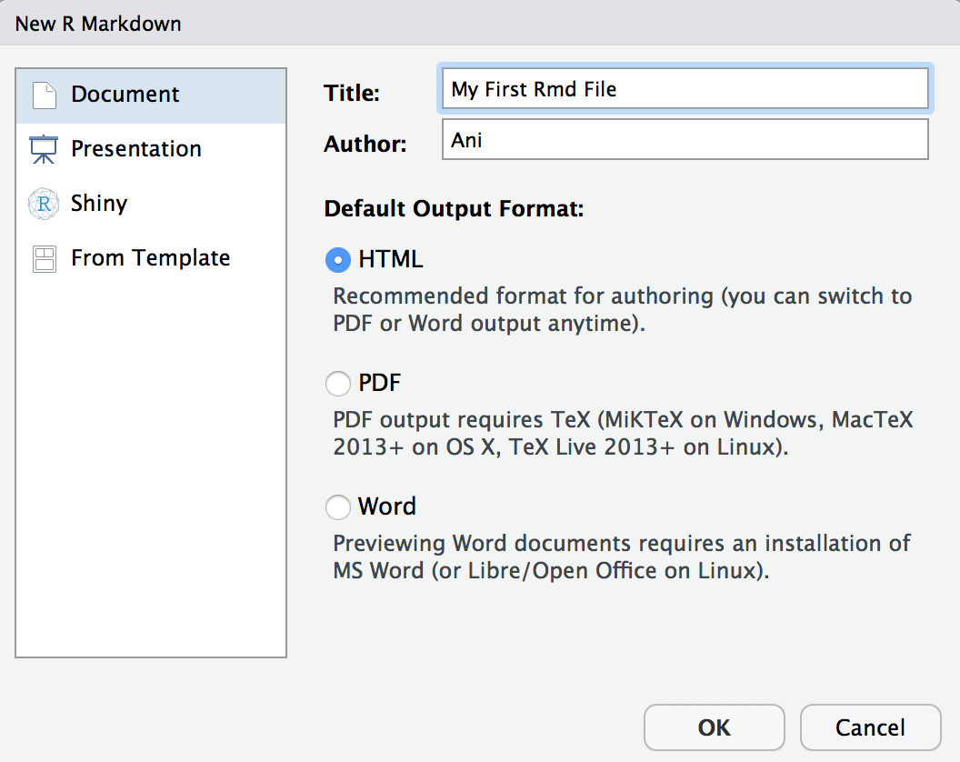
- Click
OK. - Now
File -> Save As..and save it astesting_rmdin the code sub-folder - Click this button:

You may see a message that says some packages need to be installed/updated. Allow these to be installed/updated.
... if all goes well ...
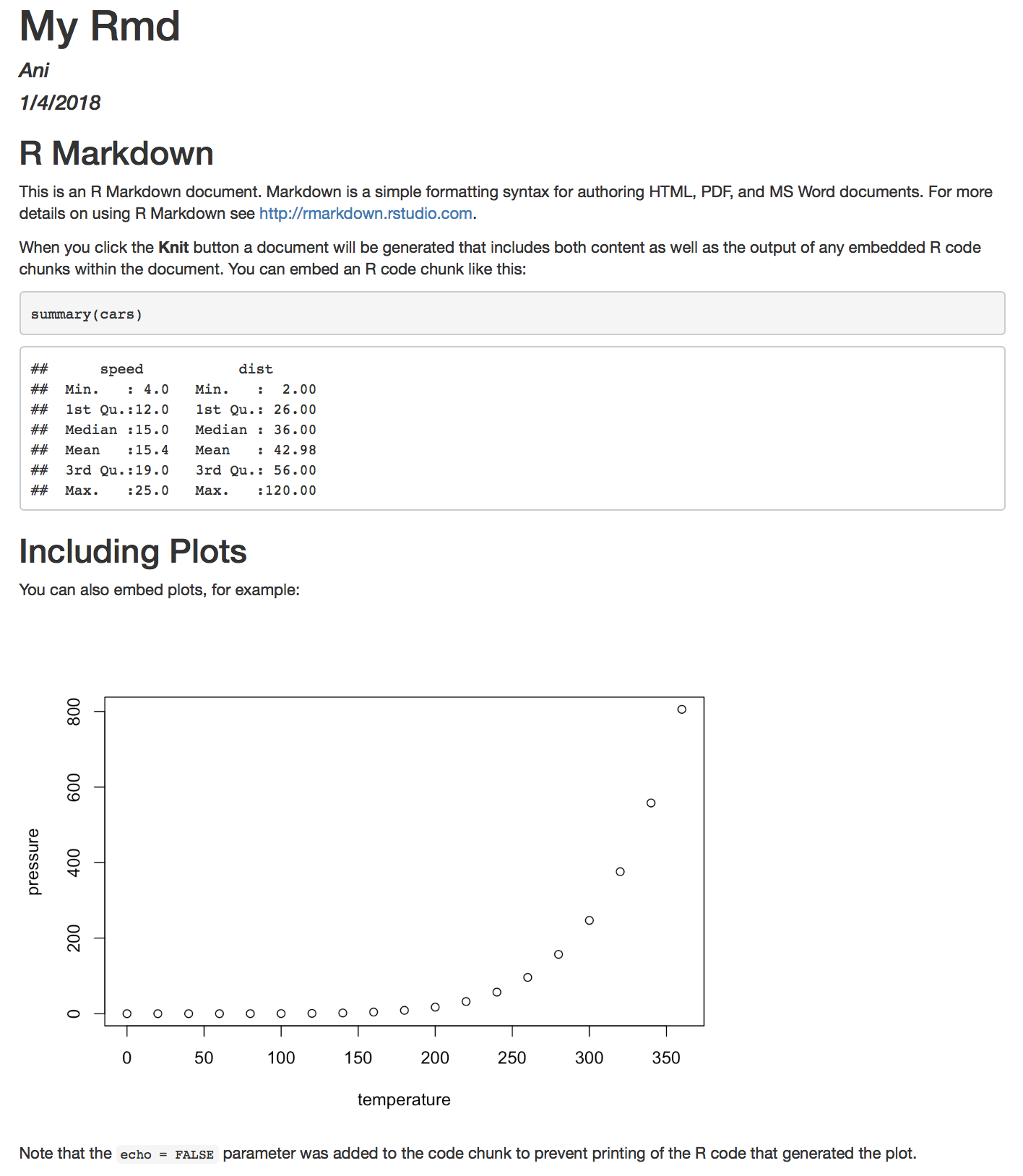
As the document knits, watch for error messages

(c) It is also common to encounter fixed-width files where the raw data are stored without any gaps between successive variables. However, these files will come with documentation that will tell you where each variable starts and ends, along with other details about each variable.
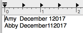
read.fwf( here("data", "fwfdata.txt"), widths = c(4, 9, 2, 4), header = FALSE, col.names = c("Name", "Month", "Day", "Year") ) -> df.fwNotice we need widths = c() and col.names = c()
save your work!!
Having added labels to the factors in hsb2 we can now save the data for later use.
save(hsb2, file = here("data", "hsb2.RData"))Let us test if this R Markdown file will  to html
If all is good then we can Close Project
- RStudio will close your project and reopen in a vanilla session
