For example, with the credit.sav dataset we could estimate the following regression model:
Rating=α+β1(Income)+β2(No. of Active Cards)+ϵ
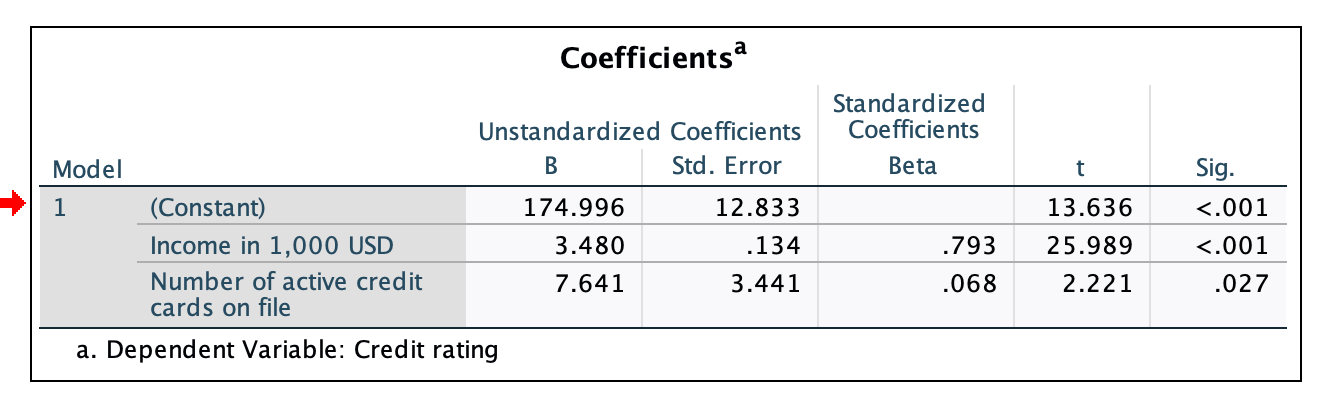
^b1=3.480: Holding the number of active cards fixed, as income increases by 1 (which is in reality an increase of 1 thousand USD), credit rating increases by about 3.48
^b2=7.641: Holding income fixed, as the number of active credit cards increases by 1, credit rating increases by 7.641
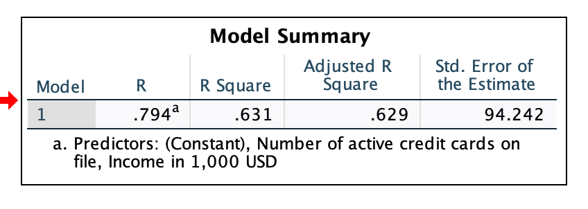
Adjusted R-Square = 0.629 ... This model predicts/explains about 62.9% of the variation in credit rating
Std. Error of the Estimate = 94.242 ... The average prediction error you can expect when using this model to predict credit ratings is ±92.242
Estimated Regression: Rating=174.996+3.48(Income)+7.641(Cards)
Since number of active cards is an integer, I would just cycle through the actual number of active cards we see in the dataset
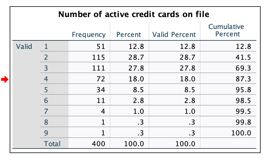
Since the upper tail is thin we may want to stop at
6
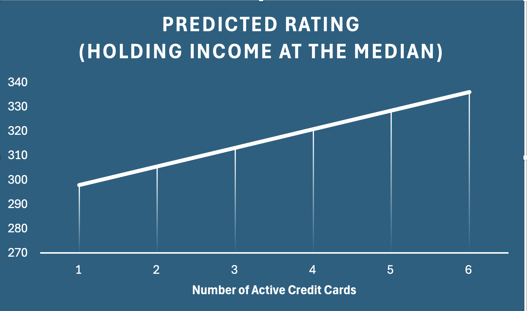
Plotting predicted ratings as number of cards increases
| Income (held fixed) | Cards | Predicted Rating |
|---|---|---|
| 33.1155 | 1 | 297.8789 |
| 33.1155 | 2 | 305.5199 |
| 33.1155 | 3 | 313.1609 |
| 33.1155 | 4 | 320.8019 |
| 33.1155 | 5 | 328.4429 |
| 33.1155 | 6 | 336.0839 |
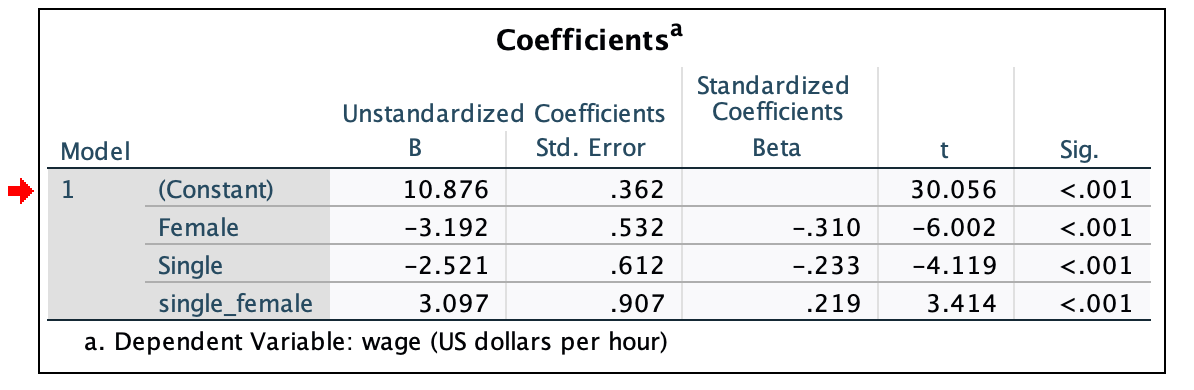
wage=a+b1(female)+b2(single)+b3(single×female)+e
Single Female: =10.876−3.192(1)−2.521(1)+3.097(1)=8.260
Married Female: =10.876−3.192(1)−2.521(0)+3.097(0)=7.684
Single Male: =10.876−3.192(0)−2.521(0)+3.097(0)=8.355
Married Male: =10.876−3.192(0)−2.521(0)+3.097(0)=10.876
The intercept is the estimated hourly wage for a married male
One Categorical and One Continuous Variable
wage=a+b1(female)+b2(age)+b3(female×age)+ϵ
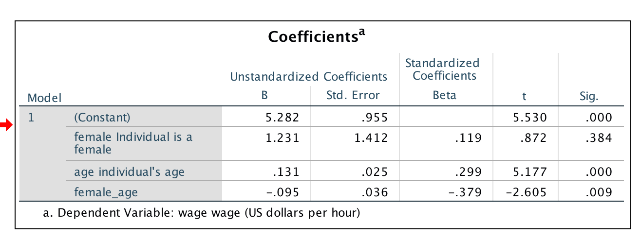
No main effect of Female (p-value = 0.384)
Main effect of age (p-value = 0.000)
Interaction effect of Female and age (p-value = 0.009) ... as age increases, the wage-gap worsens for females
Generating predicted values
Use the estimated regression model to
Calculate predicted values of wage for males with varying ages
Calculate predicted values of wage for females with the same ages you used above
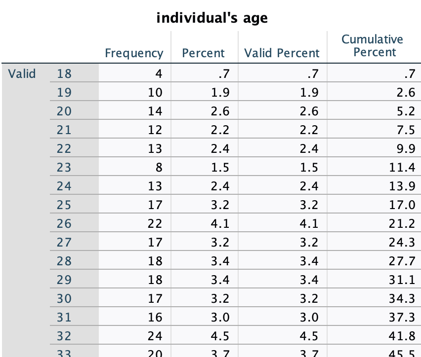
Run a frequency table for age and use the ages you see in the table
Values will be 18 through 64, in single-digit increments
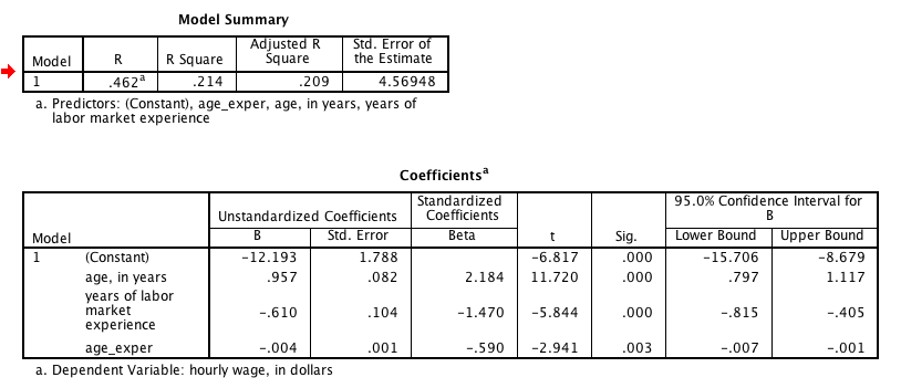
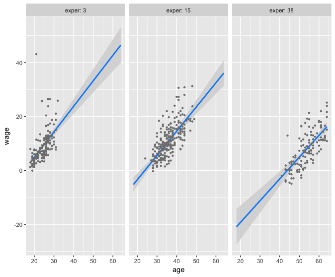
Calculate Minimum, Median, Maximum for age and for exper, respectively
Now hold age at Minimum and tweak exper
Now hold exper at Minimum and tweak age
Repeat by setting each, in turn, at Median, then at Maximum
With missing data, all descriptive statistics must be calculated for the
estimation sampleand not the full sample since if you have missing data, the descriptive statistics of the estimation sample can differ from those of the full sample

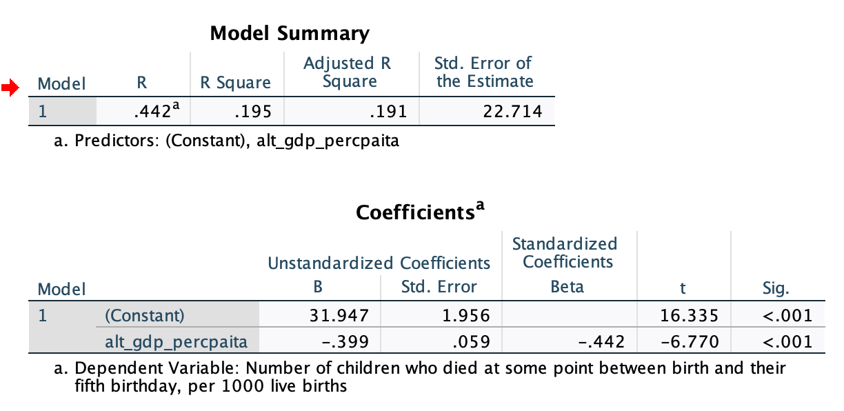
U5MR=Constant+b1(GDP)
U5MR=Constant+b1(GDP)+b2(AdultLiteracy)
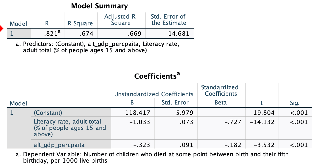
Interpret the partial slopes, adjusted R-Square, and the Standard Error of the Estimate
Notice the jump in the R-Square and the Adjusted R-Square