 from
from  from
from Understand your RStudio Environment
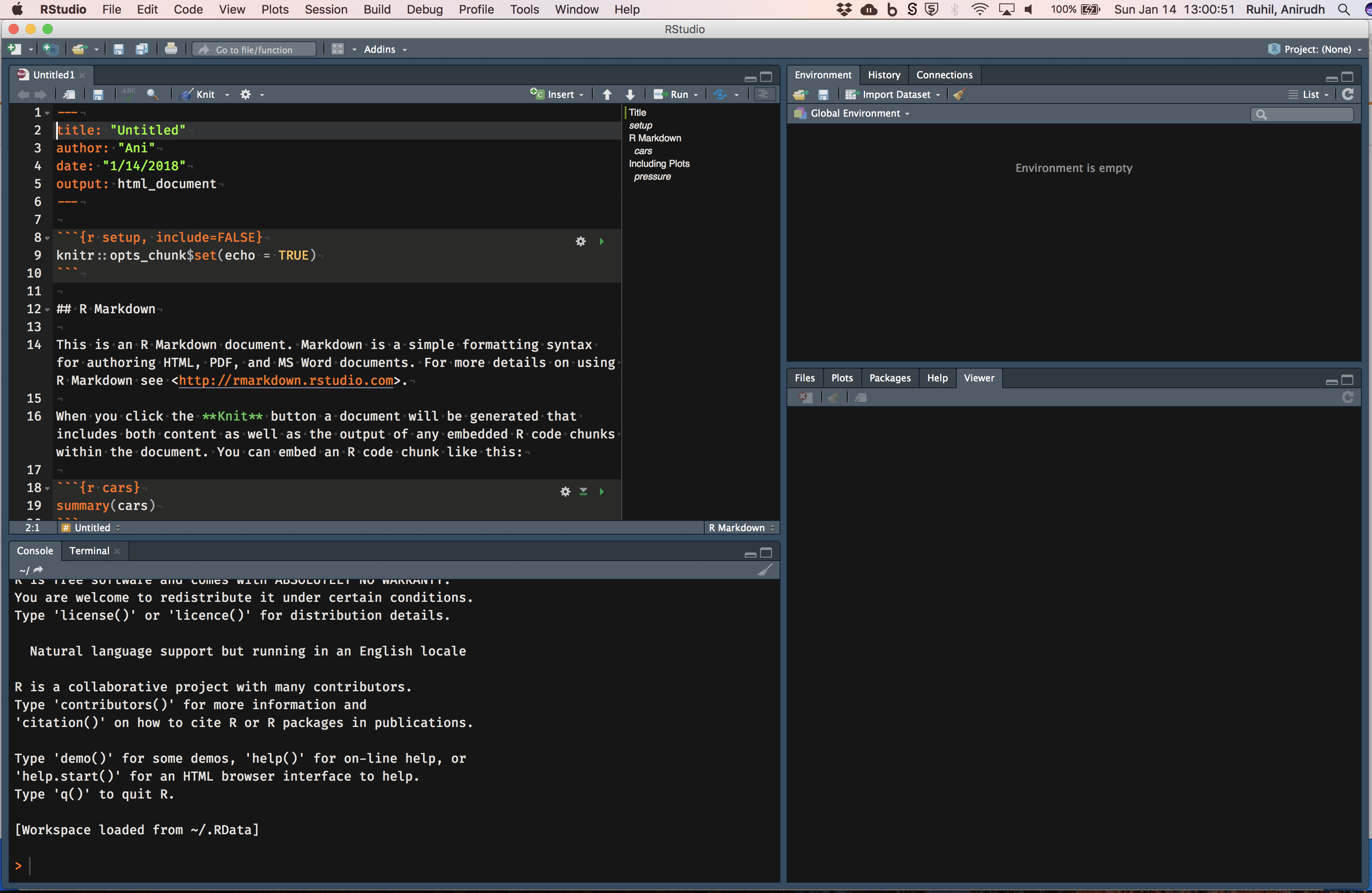
R Markdown files
- Go to
New File -> R Markdown ...and enter aMy First Rmd Filein title and yourname.
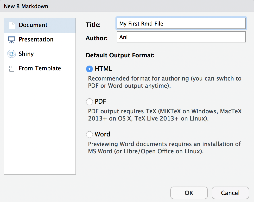
- Click
OK. - Now
File -> Save As..and save it astesting_rmdin the code sub-folder - Click this button:

You may see a message that says some packages need to be installed/updated. Allow these to be installed/updated.
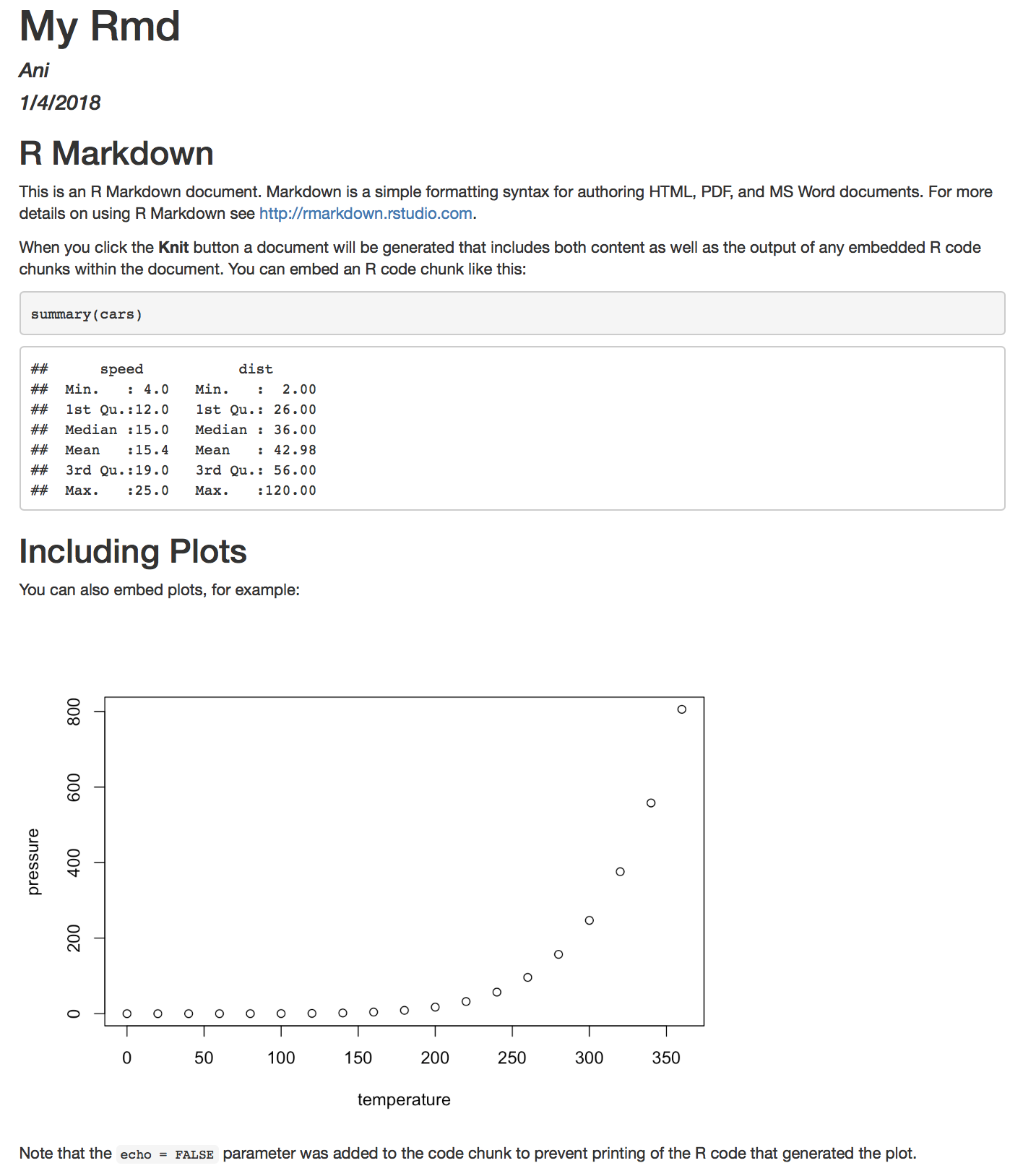
... if all goes well ...
As the document knits, watch for error messages

Excel files can be read via the readxl package
library(readxl)read_excel(here("data", "ImportDataXLS.xls")) -> df.xls read_excel(here("data", "ImportDataXLSX.xlsx")) -> df.xlsxSPSS, Stata, SAS files can be read via the haven package
library(haven)read_stata(here("data", "ImportDataStata.dta")) -> df.stata read_sas(here("data", "ImportDataSAS.sas7bdat")) -> df.sasread_sav(here("data", "ImportDataSPSS.sav")) -> df.spssFixed-width files: It is also common to encounter fixed-width files where the raw data are stored without any gaps between successive variables. However, these files will come with documentation that will tell you where each variable starts and ends, along with other details about each variable.
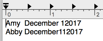
read.fwf(here("data", "fwfdata.txt"), widths = c(4, 9, 2, 4), header = FALSE, col.names = c("Name", "Month", "Day", "Year")) -> df.fwfNotice we need widths = c() and col.names = c(). We will wrestle with some fixed-width files in the coming weeks.
save your work!!
Having added labels to the factors in hsb2 we can now save the data for later use.
save(hsb2, file = "data/hsb2.RData")Let us test if this R Markdown file will to html
If all is good then we can Close Project
- RStudio will close your project and reopen in a vanilla session
Mapping in R with leaflet

Exercises for practice

Ex. 1: Creating and knitting a new RMarkdown file
Open a fresh session by launching RStudio and then running File -> Open Project...
Give it a title, your name as the author, and then save it with in code with the following name: m1ex1.Rmd
Delete all content after the following code chunk
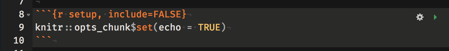
Add this level 1 heading The Starwars Data and then insert your first code chunk exactly as shown below
library(dplyr)data(starwars)str(starwars)Add this level 2 heading Character Heights and Weights and then your second code chunk
plot(starwars$height, plot$mass)Now knit this file to html
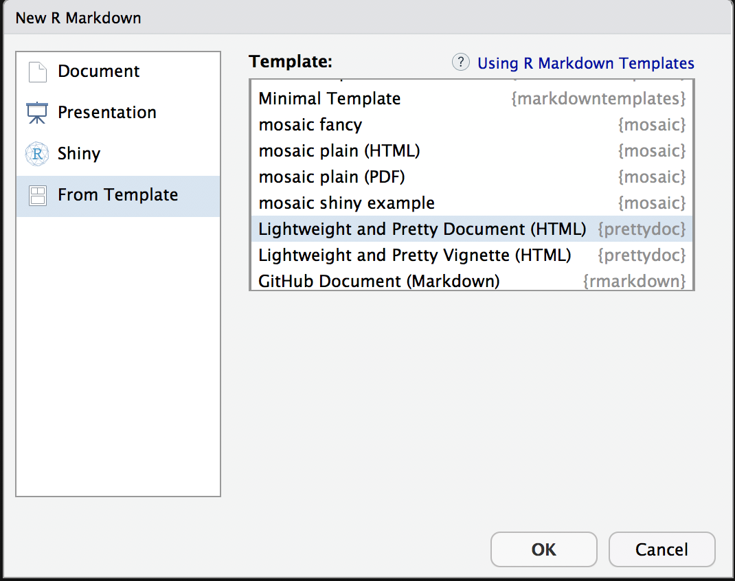
Ex. 4: Knitting with prettydoc
I'd like you to use a specific Rmd because these are very readable
You had installed the prettydoc package so now create a prettydoc Rmd file as shown below:
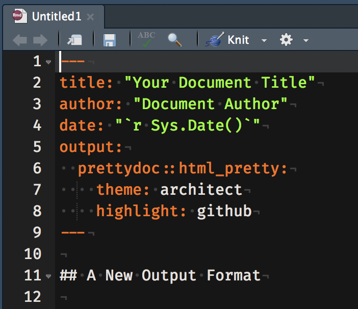
Now take all the text and code chunk you created in Ex. 3 and insert it in this file. Make sure you add a title, etc in the YAML and then knit the file to html
You can play with the theme: and highlight: fields, choosing from the options displayed here
To see native R Markdown formatting options read the documentation
