Basic Data Operations in RAni Ruhil1 / 55

Basic data operationsCommon data types and modifications 
Case operations 
Subsetting data and factor levels 
Exporting data 
Merging data 
Dealing with duplicates 
Rearranging a data-frame 
Working with strings 
2 / 55

Common data types 3 / 55

For the most part you'll focus on variables that are

numeric -- the usual quantitative measures, also called "continuous" variables
factors -- categorical variables such as sex, BMI categories, and so on
dates -- but we'll deal with these in detail later

look at the variables in the hsb data

read.table('https://stats.idre.ucla.edu/stat/data/hsb2.csv', header = TRUE, sep = ",") -> hsb
names(hsb)

##  [1] "id"      "female"  "race"    "ses"     "schtyp"  "prog"    "read"    "write"  
##  [9] "math"    "science" "socst"

str(hsb)

## 'data.frame':    200 obs. of  11 variables:
##  $ id     : int  70 121 86 141 172 113 50 11 84 48 ...
##  $ female : int  0 1 0 0 0 0 0 0 0 0 ...
##  $ race   : int  4 4 4 4 4 4 3 1 4 3 ...
##  $ ses    : int  1 2 3 3 2 2 2 2 2 2 ...
##  $ schtyp : int  1 1 1 1 1 1 1 1 1 1 ...
##  $ prog   : int  1 3 1 3 2 2 1 2 1 2 ...
##  $ read   : int  57 68 44 63 47 44 50 34 63 57 ...
##  $ write  : int  52 59 33 44 52 52 59 46 57 55 ...
##  $ math   : int  41 53 54 47 57 51 42 45 54 52 ...
##  $ science: int  47 63 58 53 53 63 53 39 58 50 ...
##  $ socst  : int  57 61 31 56 61 61 61 36 51 51 ...

4 / 55

Some of these variables are not really numeric, in particular:

female = (0/1)
race = (1=hispanic 2=asian 3=african-amer 4=white)
ses = socioeconomic status (1=low 2=middle 3=high)
schtyp = type of school (1=public 2=private)
prog = type of program (1=general 2=academic 3=vocational)

We will have to convert these pseudo-numeric variables and label what the values represent

factor(hsb$female, levels = c(0, 1), labels = c("Male", "Female")) -> hsb$female 
factor(hsb$race, levels = c(1:4), labels = c("Hispanic", "Asian", "African American", "White")) -> hsb$race 
factor(hsb$ses, levels = c(1:3), labels = c("Low", "Middle", "High")) -> hsb$ses 
factor(hsb$schtyp, levels = c(1:2), labels = c("Public", "Private")) -> hsb$schtyp 
factor(hsb$prog, levels = c(1:3), labels = c("General", "Academic", "Vocational")) -> hsb$prog 
str(hsb)

## 'data.frame':    200 obs. of  11 variables:
##  $ id     : int  70 121 86 141 172 113 50 11 84 48 ...
##  $ female : Factor w/ 2 levels "Male","Female": 1 2 1 1 1 1 1 1 1 1 ...
##  $ race   : Factor w/ 4 levels "Hispanic","Asian",..: 4 4 4 4 4 4 3 1 4 3 ...
##  $ ses    : Factor w/ 3 levels "Low","Middle",..: 1 2 3 3 2 2 2 2 2 2 ...
##  $ schtyp : Factor w/ 2 levels "Public","Private": 1 1 1 1 1 1 1 1 1 1 ...
##  $ prog   : Factor w/ 3 levels "General","Academic",..: 1 3 1 3 2 2 1 2 1 2 ...
##  $ read   : int  57 68 44 63 47 44 50 34 63 57 ...
##  $ write  : int  52 59 33 44 52 52 59 46 57 55 ...
##  $ math   : int  41 53 54 47 57 51 42 45 54 52 ...
##  $ science: int  47 63 58 53 53 63 53 39 58 50 ...
##  $ socst  : int  57 61 31 56 61 61 61 36 51 51 ...

5 / 55

If we wanted to be prudent we could have created new factors, preserving the original data (my preference and now a habit)

read.table('https://stats.idre.ucla.edu/stat/data/hsb2.csv', header = TRUE, sep = ",") -> hsb 
factor(hsb$female, levels = c(0, 1), labels = c("Male", "Female")) -> hsb$female.f 
factor(hsb$race, levels = c(1:4), labels = c("Hispanic", "Asian", "African American", "White")) -> hsb$race.f 
factor(hsb$ses, levels = c(1:3), labels = c("Low", "Middle", "High")) -> hsb$ses.f 
factor(hsb$schtyp, levels = c(1:2), labels = c("Public", "Private")) -> hsb$schtyp.f 
factor(hsb$prog, levels = c(1:3), labels = c("General", "Academic", "Vocational")) -> hsb$prog.f

6 / 55

At times, we may have numbers that get read in as characters or factors, as is evident from the example below:

c(1, 2, 3, 4, 5) -> x1 
c(1, 2, 3, 4, "a5") -> x2
c(1, 2, 3, 4, "hello") -> x3
c(1, 2, 3, 4, NA) -> x4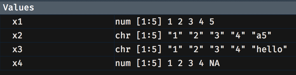

Notice that x1 and x2 are read in as numeric but x2 and x3 show up as chr, short for character. You could convert x2 and x3 into numeric as follows:

as.numeric(x2) -> x2.num 
as.numeric(x3) -> x3.num

The NA values are not applicable values, essentially missing values.

7 / 55

At times the variable may in fact be numeric but because of some anomalies in the variable, R will read it in as a factor. When this happens, converting the variable into numeric has to be done with care. Just running as.numeric() will not work. See the example below where age is flagged as a factor, perhaps because the variable was stored and exported with the double-quotation marks.

c(100, 101, 102, 103, 104, 105, 106) -> score 
c("Male", "Female", "Male", "Female", "Female", "Male", "Female") -> sex 
c("18", "18", "19", "19", "21", "21", "NA") -> age 
cbind.data.frame(score, sex, age) -> my.df

If I try as.numeric() the conversion uses the factor codings 1, 2, 3, 4 instead of the actual age values. So what is recommended is that you run as.numeric(levels(data$variable))[data$variable] instead. You can see the difference by comparing age.num1 against age.num2.

as.numeric(my.df$age) -> my.df$age.num1 
as.numeric(levels(my.df$age))[my.df$age] -> my.df$age.num2

Open up the data-frame and then see these two variables to understand how age.num1 is invalid but age.num2 is valid

8 / 55

We often need to transform an original numeric variable, stored perhaps as a proportion that we want to convert into a percentage. Or we may want to square it, divide it by 100, and so on. These operations are very straightforward.

data.frame(x = c(0.1, 0.2, 0.3, 0.4)) -> my.df 
# Convert x from proportion to percent
my.df$x * 100 -> my.df$x.pct 
# Divide x by 10
my.df$x / 10 -> my.df$x.div 
# Square x
my.df$x^2 -> my.df$x.sqrd 
# Take the square-root of x
sqrt(my.df$x) -> my.df$x.sqrt 
# Multiply x by 2
my.df$x * 2 -> my.df$x.dbled

This is the result ...

x	x%	x/10	x^2	x^(1/2)	2x
0.1	10	0.01	0.01	0.3162278	0.2
0.2	20	0.02	0.04	0.4472136	0.4
0.3	30	0.03	0.09	0.5477226	0.6
0.4	40	0.04	0.16	0.6324555	0.8

9 / 55

We can also group numeric data into bins. Let us see this with our reading scores from the hsb2 data-set.

load("data/hsb2.RData")
cut(hsb2$read, breaks = c(28, 38, 48, 58, 68, 78)) -> hsb2$grouped_read 
table(hsb2$grouped_read)

## 
## (28,38] (38,48] (48,58] (58,68] (68,78] 
##      13      69      61      47       9

Uh oh! we have a total of 199 so what happened to the 200th? The one that wasn't grouped is a reading score of 28. Why? You have to choose left-open or right-open intervals... should 38 go in the 38-48 group or the 28-38 group? This decision can be invoked by adding right = FALSE or right = TRUE (which is the default). So let me set right = FALSE.

cut(hsb2$read,
    breaks = c(28, 38, 48, 58, 68, 78),
    right = FALSE) -> hsb2$grouped_read2 
table(hsb2$grouped_read2)

## 
## [28,38) [38,48) [48,58) [58,68) [68,78) 
##      14      68      62      36      20

Open hsb2 and arrange rows in ascending order of read. Find read = 48. With the default right = TRUE 48 put in 38-48 group but with right = FALSE 48 put in 48-58 group. So right = FALSE only include values in a group (a,b] if the value is $a <= x < b$ . With right = TRUE only include values in a group [a, b) if the value is $a < x <= b$ .

10 / 55

<div id="htmlwidget-96cbf205c1d7c8d8211d" style="width:100%;height:auto;" class="datatables html-widget"></div>
<script type="application/json" data-for="htmlwidget-96cbf205c1d7c8d8211d">{"x":{"filter":"none","data":[["1","2","3","4","5","6","7","8","9","10","11","12","13","14","15","16","17","18","19","20","21","22","23","24","25","26","27","28","29","30","31","32","33","34","35","36","37","38","39","40","41","42","43","44","45","46","47","48","49","50","51","52","53","54","55","56","57","58","59","60","61","62","63","64","65","66","67","68","69","70","71","72","73","74","75","76","77","78","79","80","81","82","83","84","85","86","87","88","89","90","91","92","93","94","95","96","97","98","99","100","101","102","103","104","105","106","107","108","109","110","111","112","113","114","115","116","117","118","119","120","121","122","123","124","125","126","127","128","129","130","131","132","133","134","135","136","137","138","139","140","141","142","143","144","145","146","147","148","149","150","151","152","153","154","155","156","157","158","159","160","161","162","163","164","165","166","167","168","169","170","171","172","173","174","175","176","177","178","179","180","181","182","183","184","185","186","187","188","189","190","191","192","193","194","195","196","197","198","199","200"],[57,68,44,63,47,44,50,34,63,57,60,57,73,54,45,42,47,57,68,55,63,63,50,60,37,34,65,47,44,52,42,76,65,42,52,60,68,65,47,39,47,55,52,42,65,55,50,65,47,57,53,39,44,63,73,39,37,42,63,48,50,47,44,34,50,44,60,47,63,50,44,60,73,68,55,47,55,68,31,47,63,36,68,63,55,55,52,34,50,55,52,63,68,39,44,50,71,63,34,63,68,47,47,63,52,55,60,35,47,71,57,44,65,68,73,36,43,73,52,41,60,50,50,47,47,55,50,39,50,34,57,57,68,42,61,76,47,46,39,52,28,42,47,47,52,47,50,44,47,45,47,65,43,47,57,68,52,42,42,66,47,57,47,57,52,44,50,39,57,57,42,47,42,60,44,63,65,39,50,52,60,44,52,55,50,65,52,47,63,50,42,36,50,41,47,55,42,57,55,63],["(48,58]","(58,68]","(38,48]","(58,68]","(38,48]","(38,48]","(48,58]","(28,38]","(58,68]","(48,58]","(58,68]","(48,58]","(68,78]","(48,58]","(38,48]","(38,48]","(38,48]","(48,58]","(58,68]","(48,58]","(58,68]","(58,68]","(48,58]","(58,68]","(28,38]","(28,38]","(58,68]","(38,48]","(38,48]","(48,58]","(38,48]","(68,78]","(58,68]","(38,48]","(48,58]","(58,68]","(58,68]","(58,68]","(38,48]","(38,48]","(38,48]","(48,58]","(48,58]","(38,48]","(58,68]","(48,58]","(48,58]","(58,68]","(38,48]","(48,58]","(48,58]","(38,48]","(38,48]","(58,68]","(68,78]","(38,48]","(28,38]","(38,48]","(58,68]","(38,48]","(48,58]","(38,48]","(38,48]","(28,38]","(48,58]","(38,48]","(58,68]","(38,48]","(58,68]","(48,58]","(38,48]","(58,68]","(68,78]","(58,68]","(48,58]","(38,48]","(48,58]","(58,68]","(28,38]","(38,48]","(58,68]","(28,38]","(58,68]","(58,68]","(48,58]","(48,58]","(48,58]","(28,38]","(48,58]","(48,58]","(48,58]","(58,68]","(58,68]","(38,48]","(38,48]","(48,58]","(68,78]","(58,68]","(28,38]","(58,68]","(58,68]","(38,48]","(38,48]","(58,68]","(48,58]","(48,58]","(58,68]","(28,38]","(38,48]","(68,78]","(48,58]","(38,48]","(58,68]","(58,68]","(68,78]","(28,38]","(38,48]","(68,78]","(48,58]","(38,48]","(58,68]","(48,58]","(48,58]","(38,48]","(38,48]","(48,58]","(48,58]","(38,48]","(48,58]","(28,38]","(48,58]","(48,58]","(58,68]","(38,48]","(58,68]","(68,78]","(38,48]","(38,48]","(38,48]","(48,58]",null,"(38,48]","(38,48]","(38,48]","(48,58]","(38,48]","(48,58]","(38,48]","(38,48]","(38,48]","(38,48]","(58,68]","(38,48]","(38,48]","(48,58]","(58,68]","(48,58]","(38,48]","(38,48]","(58,68]","(38,48]","(48,58]","(38,48]","(48,58]","(48,58]","(38,48]","(48,58]","(38,48]","(48,58]","(48,58]","(38,48]","(38,48]","(38,48]","(58,68]","(38,48]","(58,68]","(58,68]","(38,48]","(48,58]","(48,58]","(58,68]","(38,48]","(48,58]","(48,58]","(48,58]","(58,68]","(48,58]","(38,48]","(58,68]","(48,58]","(38,48]","(28,38]","(48,58]","(38,48]","(38,48]","(48,58]","(38,48]","(48,58]","(48,58]","(58,68]"],["[48,58)","[68,78)","[38,48)","[58,68)","[38,48)","[38,48)","[48,58)","[28,38)","[58,68)","[48,58)","[58,68)","[48,58)","[68,78)","[48,58)","[38,48)","[38,48)","[38,48)","[48,58)","[68,78)","[48,58)","[58,68)","[58,68)","[48,58)","[58,68)","[28,38)","[28,38)","[58,68)","[38,48)","[38,48)","[48,58)","[38,48)","[68,78)","[58,68)","[38,48)","[48,58)","[58,68)","[68,78)","[58,68)","[38,48)","[38,48)","[38,48)","[48,58)","[48,58)","[38,48)","[58,68)","[48,58)","[48,58)","[58,68)","[38,48)","[48,58)","[48,58)","[38,48)","[38,48)","[58,68)","[68,78)","[38,48)","[28,38)","[38,48)","[58,68)","[48,58)","[48,58)","[38,48)","[38,48)","[28,38)","[48,58)","[38,48)","[58,68)","[38,48)","[58,68)","[48,58)","[38,48)","[58,68)","[68,78)","[68,78)","[48,58)","[38,48)","[48,58)","[68,78)","[28,38)","[38,48)","[58,68)","[28,38)","[68,78)","[58,68)","[48,58)","[48,58)","[48,58)","[28,38)","[48,58)","[48,58)","[48,58)","[58,68)","[68,78)","[38,48)","[38,48)","[48,58)","[68,78)","[58,68)","[28,38)","[58,68)","[68,78)","[38,48)","[38,48)","[58,68)","[48,58)","[48,58)","[58,68)","[28,38)","[38,48)","[68,78)","[48,58)","[38,48)","[58,68)","[68,78)","[68,78)","[28,38)","[38,48)","[68,78)","[48,58)","[38,48)","[58,68)","[48,58)","[48,58)","[38,48)","[38,48)","[48,58)","[48,58)","[38,48)","[48,58)","[28,38)","[48,58)","[48,58)","[68,78)","[38,48)","[58,68)","[68,78)","[38,48)","[38,48)","[38,48)","[48,58)","[28,38)","[38,48)","[38,48)","[38,48)","[48,58)","[38,48)","[48,58)","[38,48)","[38,48)","[38,48)","[38,48)","[58,68)","[38,48)","[38,48)","[48,58)","[68,78)","[48,58)","[38,48)","[38,48)","[58,68)","[38,48)","[48,58)","[38,48)","[48,58)","[48,58)","[38,48)","[48,58)","[38,48)","[48,58)","[48,58)","[38,48)","[38,48)","[38,48)","[58,68)","[38,48)","[58,68)","[58,68)","[38,48)","[48,58)","[48,58)","[58,68)","[38,48)","[48,58)","[48,58)","[48,58)","[58,68)","[48,58)","[38,48)","[58,68)","[48,58)","[38,48)","[28,38)","[48,58)","[38,48)","[38,48)","[48,58)","[38,48)","[48,58)","[48,58)","[58,68)"]],"container":"<table class=\"display\">\n  <thead>\n    <tr>\n      <th> <\/th>\n      <th>read<\/th>\n      <th>grouped_read<\/th>\n      <th>grouped_read2<\/th>\n    <\/tr>\n  <\/thead>\n<\/table>","options":{"columnDefs":[{"className":"dt-center","targets":[1,2,3]},{"orderable":false,"targets":0}],"filter":"top","rownames":false,"class":"compact","order":[],"autoWidth":false,"orderClasses":false}},"evals":[],"jsHooks":[]}</script>

11 / 55

More generally you'll see folks just specify the number of cuts they want.

cut(hsb2$read, breaks = 5) -> hsb2$grouped_read3 
table(hsb2$grouped_read3)

## 
##   (28,37.6] (37.6,47.2] (47.2,56.8] (56.8,66.4]   (66.4,76] 
##          14          68          48          50          20

But since age cannot include a decimal value this may be unsuitable for our purposes. Of course, we could have avoided this open/closed business of the interval by simply doing this:

cut(hsb2$read, breaks = c(25, 35, 45, 55, 65, 75, 85)) -> hsb2$grouped_read4 
table(hsb2$grouped_read4)

## 
## (25,35] (35,45] (45,55] (55,65] (65,75] (75,85] 
##       9      45      76      49      19       2

12 / 55

chop() with {santoku} 13 / 55

Say we want the reading scores grouped in 10-point intervals.

library(santoku)
chop_width(hsb$read, width = 10) -> hsb$rchop1
table(hsb$rchop1)

## 
## [28, 38) [38, 48) [48, 58) [58, 68) [68, 78) 
##       14       68       62       36       20

If you want 5, evenly-spaced intervals, which will give each group with a width of exactly $\frac{76 - 28}{5} = 9.6$

chop_evenly(hsb$read, intervals = 5) -> hsb$rchop2
table(hsb$rchop2)

## 
##   [28, 37.6) [37.6, 47.2) [47.2, 56.8) [56.8, 66.4)   [66.4, 76] 
##           14           68           48           50           20

14 / 55

What if we want equally spaced cut-points, maybe the quintiles or the quartiles, respectively??

chop_equally(hsb$read, groups = 5) -> hsb$rchop3
table(hsb$rchop3)

## 
##   [0%, 20%)  [20%, 40%)  [40%, 60%)  [60%, 80%) [80%, 100%] 
##          39          16          62          37          46

chop_equally(hsb$read, groups = 4) -> hsb$rchop4
table(hsb$rchop4)

## 
##   [0%, 25%)  [25%, 50%)  [50%, 75%) [75%, 100%] 
##          39          44          61          56

What if you want specific quantiles?

chop_quantiles(hsb$read, c(0.05, 0.25, 0.50, 0.75, 0.95)) -> hsb$rchop5
table(hsb$rchop5)

## 
##    [0%, 5%)   [5%, 25%)  [25%, 50%)  [50%, 75%)  [75%, 95%] (95%, 100%] 
##           9          30          44          61          47           9

15 / 55

Cut-points in terms of the mean and standard deviation?

chop_mean_sd(hsb$read,) -> hsb$rchop6
table(hsb$rchop6)

## 
## [-3 sd, -2 sd) [-2 sd, -1 sd)  [-1 sd, 0 sd)   [0 sd, 1 sd)   [1 sd, 2 sd)   [2 sd, 3 sd) 
##              2             22             91             39             39              7

If you want custom labels ...

chop_quantiles(
  hsb$read,
  c(0.05, 0.25, 0.50, 0.75, 0.95),
  labels = lbl_dash()
  ) -> hsb$rchop7
table(hsb$rchop7)

## 
##    0% - 5%   5% - 25%  25% - 50%  50% - 75%  75% - 95% 95% - 100% 
##          9         30         44         61         47          9

chop_quantiles(
  hsb$read,
  c(0.05, 0.25, 0.50, 0.75, 0.95),
  labels = lbl_seq("(A)")
  ) -> hsb$rchop8
table(hsb$rchop8)

## 
## (A) (B) (C) (D) (E) (F) 
##   9  30  44  61  47   9

And there you have it!

16 / 55

Changing case: lower/upper/title/sentence/etc 17 / 55

data.frame(
  sex = c("M", "F", "M", "F"), 
  NAMES = c("Andy", "Jill", "Jack", "Madison"), 
  age = c(24, 48, 72, 96)
  ) -> my.df

Maybe I want the names of the individuals to be all uppercase, or perhaps all lowercase. I can do this via:

tolower(my.df$sex) -> my.df$sex.lower 
toupper(my.df$sex) -> my.df$sex.upper

Maybe it is not the values but the column names that I want to convert to lowercase. This is easily done via

"names" -> colnames(my.df)[2]

Note: I asked for the second column's name to be changed to "names". I could have achieved the same thing by running:

data.frame(
  sex = c("M", "F", "M", "F"), 
  NAMES = c("Andy", "Jill", "Jack", "Madison"), 
  age = c(24, 48, 72, 96)
  ) -> my.df 
tolower(colnames(my.df)) -> colnames(my.df)

18 / 55

By the same logic, I could convert each column name to uppercase by typing

toupper(colnames(my.df)) -> colnames(my.df)

And then of course, using the following to change a specific column name to uppercase:

data.frame(
  sex = c("M", "F", "M", "F"), 
  NAMES = c("Andy", "Jill", "Jack", "Madison"), 
  age = c(24, 48, 72, 96)
  ) -> my.df 
toupper(colnames(my.df)[1]) -> colnames(my.df)[1] 
"AGE" -> colnames(my.df)[3]

What about title case?

c("somewhere over the rainbow", "to kill a mockingbird", "the reluctant fundamentalist") -> x 
library(tools)
toTitleCase(x) -> x.title 
x.title

## [1] "Somewhere over the Rainbow"   "To Kill a Mockingbird"       
## [3] "The Reluctant Fundamentalist"

When we work with stringi and stringr we'll see other ways of switching letter cases

19 / 55

A little bit about factors 20 / 55

With the hsb data we created some factors. Here I want to show you a couple of things to pay attention to.

First, I can create a new variable and store it as a factor as follows:

my.df$female1[my.df$SEX == "M"] = 1 
my.df$female1[my.df$SEX == "F"] = 2 
factor(
  my.df$female1,
  levels = c(1, 2),
  labels = c("Male", "Female")
  ) -> my.df$female1

I could have also skipped the 0/1 business and just done this:

my.df$female2[my.df$SEX == "M"] = "Male"
my.df$female2[my.df$SEX == "F"] = "Female"
factor(my.df$female2) -> my.df$female2

Notice the difference between female1 and female2

female1: Since you specified levels = c(0, 1) and indicated the lowest level be mapped to Male, the factor is built in that order ... Male first, then Female
female2: Here we did not specify the levels and hence R falls back on its default of building them up alphabetically ... Female first, then Male

21 / 55

Let us see factor levels with a different example. Say we had the following variable, 10 responses to a survey question.

data.frame(x = c(
  rep("Disagree", 3),
  rep("Neutral", 2),
  rep("Agree", 5)
  )
  ) -> fdf 
factor(fdf$x) -> fdf$responses 
levels(fdf$responses)

## [1] "Agree"    "Disagree" "Neutral"

table(fdf$responses)

## 
##    Agree Disagree  Neutral 
##        5        3        2

22 / 55

This makes no sense since we'd like the logical ordering of Disagree -> Neutral -> Agree

ordered(
  fdf$responses,
  levels = c("Disagree", "Neutral", "Agree")
  ) -> fdf$newresponses 
levels(fdf$newresponses)

## [1] "Disagree" "Neutral"  "Agree"

min(fdf$newresponses)

## [1] Disagree
## Levels: Disagree < Neutral < Agree

table(fdf$newresponses)

## 
## Disagree  Neutral    Agree 
##        3        2        5

23 / 55

I could have also generated this desired order when creating the factor as, for example, via

factor(fdf$x,
       ordered = TRUE,
       levels = c("Disagree", "Neutral", "Agree")
       ) -> fdf$xordered 
levels(fdf$xordered)

## [1] "Disagree" "Neutral"  "Agree"

min(fdf$xordered)

## [1] Disagree
## Levels: Disagree < Neutral < Agree

table(fdf$xordered)

## 
## Disagree  Neutral    Agree 
##        3        2        5

Notice the min() command ... which asks for the minimum level of a factor. This works with ordered factors but not with unordered factors; try it with x and with responses.

24 / 55

Before we move on, a word about the command we used to generate a new factor from an existing variable

"Male" -> my.df$female2[my.df$SEX == "M"] 
"Female" -> my.df$female2[my.df$SEX == "F"]

You may run into this a lot when generating new variables, and even when fixing problems with an existing variable. For example, say we were given the data on the sex of these 10 individuals but the values included typos.

data.frame(
  mf = c(
    rep("Male", 3),
    rep("male", 2),
    rep("Female", 3),
    rep("femalE", 2)
    )
  ) -> sexdf 
sexdf$mf = factor(sexdf$mf)
levels(sexdf$mf)

## [1] "femalE" "Female" "male"   "Male"

25 / 55

Obviously not what we'd like so we can go in and clean it up a bit. How? As follows:

"Male" -> sexdf$mf[sexdf$mf == "male"] 
"Female" -> sexdf$mf[sexdf$mf == "femalE"] 
levels(sexdf$mf)

## [1] "femalE" "Female" "male"   "Male"

table(sexdf$mf)

## 
## femalE Female   male   Male 
##      0      5      0      5

26 / 55

Wait a second, we still see femalE and male but with 0 counts; how should we get rid of these ghosts?

droplevels(sexdf$mf) -> sexdf$newmf 
levels(sexdf$newmf)

## [1] "Female" "Male"

table(sexdf$newmf)

## 
## Female   Male 
##      5      5

Having fixed this issue we can drop the original variable via

NULL -> sexdf$mf

27 / 55

Subsetting data and factor levels 28 / 55

What if want only a susbet of the data? For example, say I am working with the diamond data-set and need to subset my analysis to diamonds that are Very Good or better.

library(ggplot2)
data(diamonds)
str(diamonds$cut)

##  Ord.factor w/ 5 levels "Fair"<"Good"<..: 5 4 2 4 2 3 3 3 1 3 ...

table(diamonds$cut)

## 
##      Fair      Good Very Good   Premium     Ideal 
##      1610      4906     12082     13791     21551

I can subset as follows:

subset(diamonds, cut != "Fair" & cut != "Good") -> dia.sub1 
str(dia.sub1$cut)

##  Ord.factor w/ 5 levels "Fair"<"Good"<..: 5 4 4 3 3 3 3 5 4 5 ...

table(dia.sub1$cut)

## 
##      Fair      Good Very Good   Premium     Ideal 
##         0         0     12082     13791     21551

29 / 55

Aha! I see no diamonds in the excluded cut ratings but str() still shows R remembering cut as having 5 ratings and the frequency table shows up with zero counts for both so we drop these levels explicitly.

droplevels(dia.sub1$cut) -> dia.sub1$cutnew 
str(dia.sub1$cutnew)

##  Ord.factor w/ 3 levels "Very Good"<"Premium"<..: 3 2 2 1 1 1 1 3 2 3 ...

table(dia.sub1$cutnew)

## 
## Very Good   Premium     Ideal 
##     12082     13791     21551

30 / 55

Now a bit more on sub-setting data. You can subset with as simple or as complicated a condition you need. For example, maybe you only want Ideal diamonds with a certain minimum clarity and price.

subset(diamonds, cut == "Ideal" & clarity == "VVS1" & price > 3933) -> dia.sub2 
table(dia.sub2$cut)

## 
##      Fair      Good Very Good   Premium     Ideal 
##         0         0         0         0       283

table(dia.sub2$clarity)

## 
##   I1  SI2  SI1  VS2  VS1 VVS2 VVS1   IF 
##    0    0    0    0    0    0  283    0

min(dia.sub2$price)

## [1] 3955

Here the sub-setting is generating a data-frame that will only include observations that meet all three requirements (since you used & in the command). If you had run the following instead you would have had very different results.

subset(diamonds, cut == "Ideal" | clarity == "VVS1" | price > 3933) -> dia.sub3 
subset(diamonds, cut == "Ideal" & clarity == "VVS1" | price > 3933) -> dia.sub4 
subset(diamonds, cut == "Ideal" | clarity == "VVS1" & price > 3933) -> dia.sub5

31 / 55

Exporting data 32 / 55

Often, after data have been processed in R, we need to share them with folks who don't use R or want the data in a specific format. This is easily done, as shown below.

data.frame(
  Person = c("John", "Timothy", "Olivia", "Sebastian", "Serena"),
  Age = c(22, 24, 18, 24, 35)
  ) -> out.df 
write.csv(out.df, file = "data/out.csv", row.names = FALSE) # CSV format 
library(haven)
write_dta(out.df, "out.df.dta") # Stata format
write_sav(out.df, "out.df.sav") # SPSS format 
write_sas(out.df, "data/out.df.sas") # SAS format 
library(writexl)
write_xlsx(out.df, "data/out.df.xlsx") # Excel format

There are other packages that import/export data so be sure to check them out as well, in particular rio.

33 / 55

Merging data 34 / 55

Say I have data on some students, with test scores in one file and their gender in another file. Each file has a unique student identifier, called ID. How can I create a single data-set? Let us see each data-set first.

data.frame(
  Score = c(10, 21, 33, 12, 35, 67, 43, 99),
  ID = c("A12", "A23", "Z14", "WX1", "Y31", "D66", "C31", "Q22")
  ) -> data1 
data.frame(
  Sex = c("Male", "Female", "Male", "Female", "Male", "Female", "Male", "Female"),
  ID = c("A12", "A23", "Z14", "WX1", "Y31", "D66", "E52", "H71")
  ) -> data2

Open up both data-sets and note that students C31 and Q22 are missing from data2 and students E52 and H71 are missing from data1.

35 / 55

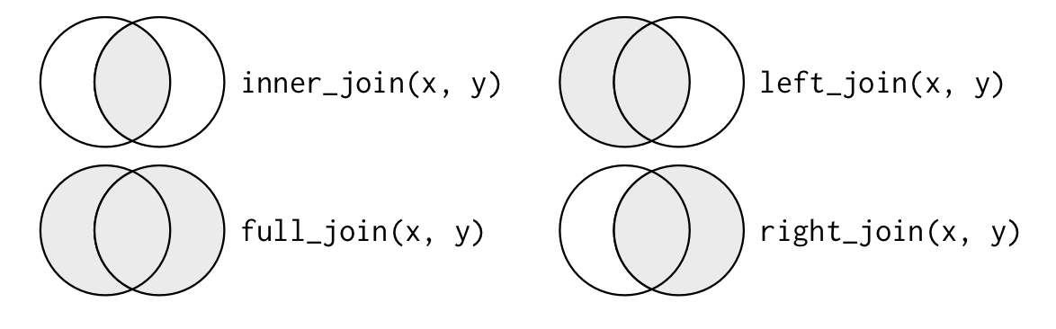
... here are the two data-sets<div id="htmlwidget-b171b565011c082c9d51" style="width:100%;height:auto;" class="datatables html-widget"></div>
<script type="application/json" data-for="htmlwidget-b171b565011c082c9d51">{"x":{"filter":"none","data":[["1","2","3","4","5","6","7","8"],[10,21,33,12,35,67,43,99],["A12","A23","Z14","WX1","Y31","D66","C31","Q22"]],"container":"<table class=\"display\">\n  <thead>\n    <tr>\n      <th> <\/th>\n      <th>Score<\/th>\n      <th>ID<\/th>\n    <\/tr>\n  <\/thead>\n<\/table>","options":{"columnDefs":[{"className":"dt-center","targets":[1,2]},{"orderable":false,"targets":0}],"filter":"top","rownames":false,"class":"compact","order":[],"autoWidth":false,"orderClasses":false}},"evals":[],"jsHooks":[]}</script>

<div id="htmlwidget-bcf4d900b28a98d02dfa" style="width:100%;height:auto;" class="datatables html-widget"></div>
<script type="application/json" data-for="htmlwidget-bcf4d900b28a98d02dfa">{"x":{"filter":"none","data":[["1","2","3","4","5","6","7","8"],["Male","Female","Male","Female","Male","Female","Male","Female"],["A12","A23","Z14","WX1","Y31","D66","E52","H71"]],"container":"<table class=\"display\">\n  <thead>\n    <tr>\n      <th> <\/th>\n      <th>Sex<\/th>\n      <th>ID<\/th>\n    <\/tr>\n  <\/thead>\n<\/table>","options":{"columnDefs":[{"className":"dt-center","targets":[1,2]},{"orderable":false,"targets":0}],"filter":"top","rownames":false,"class":"compact","order":[],"autoWidth":false,"orderClasses":false}},"evals":[],"jsHooks":[]}</script>

36 / 55

What about the merge? To merge data-frames we need to specify the merge key(s) -- the variable(s) that identifies unique observations in each file. This variable(s) must be present in all the files you want to merge. So long as it exists, you now need to decide: Do you only want to

merge observations that show up in both files (natural join)
merge everything even if some cases show up in one but not the other (full outer join)
merge such that all cases in file x are retained but only those seen in file y are joined (left outer join)
merge to keep all cases in y and only those cases are to be merged from x that show up in y, referred to as (right outer join)

merge(x = data1, y = data2, by = c("ID"), all = FALSE) -> natural   # only merge if ID seen in both files
merge(x = data1, y = data2, by = c("ID"), all = TRUE) -> full # merge everything 
merge(x = data1, y = data2, by = c("ID"), all.x = TRUE) -> left # make sure all cases from file x are retained 
merge(x = data1, y = data2, by = c("ID"), all.y  = TRUE) -> right # make sure all cases from file y are retained

Garrett and Hadley have a wonderful chapter on joins and the diagram below is one of their many descriptors.

37 / 55

What if the ID variables had different names in the files? You could rename them to have a common name or you could use by.x = and by.y = as shown below.

data.frame(
  Score = c(10, 21, 33, 12, 35, 67, 43, 99),
  ID1 = c("A12", "A23", "Z14", "WX1", "Y31", "D66", "C31", "Q22")
  ) -> data3 
data.frame(
  Sex = c("Male", "Female", "Male", "Female", "Male", "Female", "Male", "Female"),
  ID2 = c("A12", "A23", "Z14", "WX1", "Y31", "D66", "E52", "H71")
  ) -> data4 
merge(
  data3, data4, 
  by.x = c("ID1"),
  by.y = c("ID2"),
  all = FALSE
  ) -> diffids

You can also have more than one merge key. For example, if I am merging data for Ohio schools, each district has a district ID number (dirn), each school has building ID number (birn), and then the district's name (district), the building's name (building), and so on. If I am merging these data then my by = statement will be by = c("dirn", "birn", "district", "building").

38 / 55

If we have multiple data-frames to merge we can do so in several ways but my default approach is to rely on the Reduce() command, as shown below.

data.frame(
  Score = c(10, 21, 33, 12, 35, 67, 43, 99),
  ID = c("A12", "A23", "Z14", "WX1", "Y31", "D66", "C31", "Q22")
  ) -> df1 
data.frame(
  Sex = c("Male", "Female", "Male", "Female", "Male", "Female", "Male", "Female"),
  ID = c("A12", "A23", "Z14", "WX1", "Y31", "D66", "E52", "H71")
  ) -> df2 
data.frame(
  Age = c(6, 7, 6, 8, 8, 9, 10, 5),
  ID = c("A12", "A23", "Z14", "WX1", "Y31", "D66", "E52", "H71")
  ) -> df3 
list(df1, df2, df3) -> my.list 
Reduce(function(...) merge(..., by = c("ID"), all = TRUE), my.list) -> df.123

39 / 55

Here is the merged data-frame ...

ID	Score	Sex	Age
A12	10	Male	6
A23	21	Female	7
C31	43	NA	NA
D66	67	Female	9
E52	NA	Male	10
H71	NA	Female	5
Q22	99	NA	NA
WX1	12	Female	8
Y31	35	Male	8
Z14	33	Male	6

40 / 55

Dealing with duplicates 41 / 55

Every now and then you also run into duplicate rows with no good explanation for how that could have happened. Here is an example:

data.frame(
  Sex = c("Male", "Female", "Male", "Female", "Male", "Female", "Male", "Female"),
  ID = c("A12", "A23", "Z14", "WX1", "Y31", "D66", "A12", "WX1")
  ) -> dups.df

Students A12 and WX1 show up twice! There are two basic commands that we can use to find duplicates -- unique and duplicated.

duplicated(dups.df) # flag duplicate rows with TRUE 
!duplicated(dups.df) # flag not duplicated rows with TRUE 
dups.df[duplicated(dups.df), ] # reveal the duplicated rows 
dups.df[!duplicated(dups.df), ] # reveal the not duplicated rows 
dups.df[!duplicated(dups.df), ] -> nodups.df # save a dataframe without duplicated rows
dups.df[duplicated(dups.df), ] -> onlydups.df # save a dataframe with ONLY the duplicated rows

42 / 55

Rearranging the data-set 43 / 55

We may, at times, want to move the variables around so they are in a particular order (age next to race and so on, for example), perhaps drop some because there are too many variables and we don't need all of them. We may also want to arrange the data-frame in ascending or descending order of some variable(s) (increasing order of age or price for example.

mtcars[order(mtcars$mpg), ] -> df1 # arrange the data-frame in ascending order of mpg 
mtcars[order(-mtcars$mpg), ] -> df2 # arrange the data-frame in descending order of mpg
mtcars[order(mtcars$am, mtcars$mpg), ] -> df3 # arrange the data-frame in ascending order of automatic/manual and then in ascending order of mpg

What if I want to order the columns such that the first column is am and then comes mpg, followed by qsec and then the rest of the columns? Well, the first thing I want to do is see what variable is in which column via the names() command.

names(mtcars) # the original structure of the mtcars data-frame

##  [1] "mpg"  "cyl"  "disp" "hp"   "drat" "wt"   "qsec" "vs"   "am"   "gear" "carb"

So mpg is in column 1, cyl is in column 2, and carb is the last one in column 11.

Now I'll specify that I want all rows by doing this [, c()] and then specify the order of the columns by entering the column numbers in c()

mtcars[, c(9, 1, 7, 2:6, 8, 10:11)] -> df4 # specifying the position of the columns 
names(df4)

##  [1] "am"   "mpg"  "qsec" "cyl"  "disp" "hp"   "drat" "wt"   "vs"   "gear" "carb"

44 / 55

If I only wanted certain columns I could simply not list the other columns.

mtcars[, c(9, 1, 7)] -> df5 # specifying the position of the columns

Remember the comma in mtcars[, ... this tells R to keep all rows in mtcars. If, instead, I did this I would only get the first four rows, not all.

mtcars[1:4, c(9, 1, 7)] -> df6 # keep first four rows and the specified columns

I would end up with only the first four rows of mtcars, not every row. So try to remember the order: dataframe[i, j] where i reference the rows and j reference the columns.

45 / 55

Working with strings 46 / 55

Often you run into strings that have to be manipulated. Often, when working with county data, for example, county names are followed by County, Ohio and this is superfluous so we end up excising it

read.csv("data/strings.csv") -> c.data 
head(c.data)

##           GEO.id GEO.id2      GEO.display.label respop72016
## 1 0500000US39001   39001     Adams County, Ohio       27907
## 2 0500000US39003   39003     Allen County, Ohio      103742
## 3 0500000US39005   39005   Ashland County, Ohio       53652
## 4 0500000US39007   39007 Ashtabula County, Ohio       98231
## 5 0500000US39009   39009    Athens County, Ohio       66186
## 6 0500000US39011   39011  Auglaize County, Ohio       45894

Let us just retain the county name from GEO.display.label

gsub(" County, Ohio", "", c.data$GEO.display.label) -> c.data$county 
head(c.data[, c(3, 5)])

##        GEO.display.label    county
## 1     Adams County, Ohio     Adams
## 2     Allen County, Ohio     Allen
## 3   Ashland County, Ohio   Ashland
## 4 Ashtabula County, Ohio Ashtabula
## 5    Athens County, Ohio    Athens
## 6  Auglaize County, Ohio  Auglaize

Note the sequence gsub("look for this pattern", "replace with this pattern", mydata$myvariable)

47 / 55

`with` and `within`

If you need to add variables to an existing data frame, you can do it in several ways:

data.frame(x = seq(0, 5, by = 1), y = seq(10, 15, by = 1)) -> dfw 
dfw$x * dfw$y -> dfw$xy1 # the most basic creation of xy 
with(dfw, x * y) -> dfw$xy2 # using with
within(dfw, xy3 <- x * y) -> dfw # using within

x	y	xy1	xy2	xy3
0	10	0	0	0
1	11	11	11	11
2	12	24	24	24
3	13	39	39	39
4	14	56	56	56
5	15	75	75	75

Notice that if using within() the variable name must be specified as in xy3 <- x * y

48 / 55

`ifelse` and `grepl`

The ifelse command is a useful one when creating new variables (invariable factors) from an existing variable

The long way ...

data(mtcars)
mtcars$automatic2[mtcars$am == 1] = "Automatic" 
mtcars$automatic2[mtcars$am == 0] = "Manual"

The more efficient way ...

ifelse(mtcars$am == 1, "Automatic", "Manual") -> mtcars$automatic

If you have strings, then grepl comes into play:

load("data/movies.RData")
ifelse(grepl("Comedy", movies$genres), "Yes", "No") -> movies$comedy 
ifelse(grepl("(1995)", movies$title), "Yes", "No") -> movies$in1995 
ifelse(grepl("Night", movies$title), "Yes", "No") -> movies$night

In short, the function looks for the specified string (“Comedy”) in genres and if found adds a flag of “Yes” and if not found adds a flag of “No”

49 / 55

But what if I wanted to run more complicated expressions, for example if the words “Night” or “Dark” or “Cool” are used in the title?

ifelse(
  grepl("Night", movies$title), "Yes",
  ifelse(grepl("Dark", movies$title), "Yes",
         ifelse(grepl("Cool", movies$title), "Yes", "No"))
  ) -> movies$tricky

Ah grepl, you beauty!! Nesting our way to what we want ...

grep() and grepl() differ in that both functions find patterns but return different output types

grep() returns numeric values that index the locations where the patterns were found
grepl() returns a logical vector in which TRUE represents a pattern match and FALSE does not

Run the two commands that follow and focus on the output that scrolls in the console

grep("Comedy", movies$genres)
grepl("Comedy", movies$genres)

50 / 55

You could use both for sub-setting data as well.

movies[grep("Comedy", movies$genres), ] -> mov1 
movies[-grep("Comedy", movies$genres), ] -> mov2

Say I only want columns that have the letter “t” in them. No problem:

movies[, grep("t", colnames(movies))] -> mov3 # keep if t is in column name 
movies[, -grep("t", colnames(movies))] -> mov4 # keep if t is not in column name

Try using grepl instead of grep with the preceding two commands and see what results ...

movies[, grepl("t", colnames(movies))] -> mov3 
movies[, -grepl("t", colnames(movies))] -> mov4

51 / 55

sums and means 52 / 55

data.frame(
  x = c(0, 1, 2, 3, 4, NA),
  y = c(10, 11, 12, NA, 14, 15)
  ) -> dfs 
dfs

##    x  y
## 1  0 10
## 2  1 11
## 3  2 12
## 4  3 NA
## 5  4 14
## 6 NA 15

rowSums() for each row, sum the columns so that you end up with a row total

rowSums(dfs, na.rm = TRUE)  # sum columns 1 and 2 for each row

## [1] 10 12 14  3 18 15

colSums() for each column, calculate the sum of its values

colSums(dfs, na.rm = TRUE)

##  x  y 
## 10 62

53 / 55

rowMeans() for each row, calculate the mean of the columns

rowMeans(dfs, na.rm = TRUE)

## [1]  5  6  7  3  9 15

colMeans() for each column, calculate the mean

colMeans(dfs, na.rm = TRUE)

##    x    y 
##  2.0 12.4

54 / 55

Find me at...

@aruhil
aniruhil.org
ruhil@ohio.edu

55 / 55

Help

Keyboard shortcuts

↑, ←, Pg Up, k

Go to previous slide

↓, →, Pg Dn, Space, j

Go to next slide

Home

Go to first slide

End

Go to last slide

Number + Return

Go to specific slide

b / m / f

Toggle blackout / mirrored / fullscreen mode

Clone slideshow

Toggle presenter mode

Restart the presentation timer

?, h

Toggle this help

Basic Data Operations in R

Ani Ruhil

Basic data operations

Common data types

chop() with {santoku}

Changing case: lower/upper/title/sentence/etc

A little bit about factors

Subsetting data and factor levels

Exporting data

Merging data

... here are the two data-sets

Dealing with duplicates

Rearranging the data-set

Working with strings

with and within

ifelse and grepl

sums and means

Find me at...

Basic data operations

Help

`with` and `within`

`ifelse` and `grepl`