dplyr and tidyr
Ani Ruhil


"dplyr is a grammar of data manipulation, providing a consistent set of verbs that help you solve the most common data manipulation challenges"
The core functions are:
- mutate() ... to add new variables that are functions of existing variables
- transmute() ... to add new variables and drop the rest
- select() ... to pick variables (based on their names) to work on
- filter() ... to pick cases (based on their values) to work on
- summarise() .. to calculate quantities of interest (rather than add these quantities to the existing data frame) and save these as a standalone object
- arrange() ... order the rows based on out preferences
In order to understand how these commands work we rely on a simple data frame -- all flights originating and departing from Columbus (Ohio) January through September of 2017. Let us load the data and dplyr.
library(here)load("data/cmhflights2017.RData")library(dplyr)library(tidylog)select
Say I only want the first five columns.
cmhflights2017 %>% select(Year:DayOfWeek) -> my.df names(my.df)## [1] "Year" "Quarter" "Month" "DayofMonth" "DayOfWeek"What if the columns were not sequentially located?
cmhflights2017 %>% select(Year, FlightDate:DOT_ID_Reporting_Airline, Tail_Number) -> my.df names(my.df)## [1] "Year" "FlightDate" "Reporting_Airline" ## [4] "DOT_ID_Reporting_Airline" "Tail_Number"Could we use column numbers instead?
cmhflights2017 %>% select(c(1, 3, 5, 7)) -> my.df names(my.df)## [1] "id" "Quarter" "DayofMonth" "FlightDate"What about columns that cotain a specific string?
cmhflights2017 %>% select(contains("Origin")) -> my.df names(my.df)## [1] "OriginAirportID" "OriginAirportSeqID" "OriginCityMarketID" "Origin" ## [5] "OriginCityName" "OriginState" "OriginStateFips" "OriginStateName" ## [9] "OriginWac"Columns that start or end with some string?
cmhflights2017 %>% select(starts_with("De")) -> my.df names(my.df)## [1] "DestAirportID" "DestAirportSeqID" "DestCityMarketID" ## [4] "Dest" "DestCityName" "DestState" ## [7] "DestStateFips" "DestStateName" "DestWac" ## [10] "DepTime" "DepDelay" "DepDelayMinutes" ## [13] "DepDel15" "DepartureDelayGroups" "DepTimeBlk"cmhflights2017 %>% select(ends_with("Num")) -> my.df names(my.df)## [1] "Div1TailNum" "Div2TailNum" "Div3TailNum" "Div4TailNum" "Div5TailNum"Say you have columns named something like "V0124", "V0125" and so on until "V1800"; SPSS files from some data archives tend to have this naming convention. In that case, you could do:
somedata %>% select(num_range("V", 51:231)) -> my.dfdplyr also has one_of and matches as, for example, in
cmhflights2017 %>% select(one_of("Year", "Quarter", "Month", "Dest")) -> my.df names(my.df)## [1] "Year" "Quarter" "Month" "Dest"cmhflights2017 %>% select(matches("Wheels")) -> my.df names(my.df)## [1] "WheelsOff" "WheelsOn" "Div1WheelsOn" "Div1WheelsOff" "Div2WheelsOn" ## [6] "Div2WheelsOff" "Div3WheelsOn" "Div3WheelsOff" "Div4WheelsOn" "Div4WheelsOff"## [11] "Div5WheelsOn" "Div5WheelsOff"filter
We used subset() to select particular cases for analysis. With dplyr, the filter() command serves the same purpose. Say we only want records from January, i.e., Month == 1.
cmhflights2017 %>% filter(Month == 1) -> my.df table(my.df$Month)## ## 1 ## 3757What about only American Airline flights in January?
cmhflights2017 %>% filter(Month == 1 & Reporting_Airline == "AA") -> my.df table(my.df$Month, my.df$Reporting_Airline)## ## AA## 1 387What about United Airlines flights in January to CMH (Columbus, OH) to any destination?
cmhflights2017 %>% filter(Month == 1 & Reporting_Airline == "UA" & Dest == "CMH") -> my.df<div id="htmlwidget-d5995c8e0aa77f45a50e" style="width:100%;height:auto;" class="datatables html-widget"></div><script type="application/json" data-for="htmlwidget-d5995c8e0aa77f45a50e">{"x":{"filter":"none","data":[["1","2","3","4","5","6","7","8","9","10","11","12","13","14","15","16","17","18","19","20","21","22","23","24","25","26","27","28","29","30","31","32","33","34","35","36","37","38","39","40","41","42","43","44","45","46","47","48","49","50","51","52","53"],["2017-01-22","2017-01-21","2017-01-20","2017-01-20","2017-01-19","2017-01-19","2017-01-18","2017-01-04","2017-01-04","2017-01-04","2017-01-03","2017-01-03","2017-01-02","2017-01-02","2017-01-31","2017-01-31","2017-01-30","2017-01-30","2017-01-29","2017-01-28","2017-01-27","2017-01-27","2017-01-13","2017-01-13","2017-01-12","2017-01-12","2017-01-11","2017-01-11","2017-01-10","2017-01-10","2017-01-09","2017-01-09","2017-01-18","2017-01-17","2017-01-17","2017-01-16","2017-01-16","2017-01-15","2017-01-14","2017-01-26","2017-01-26","2017-01-25","2017-01-25","2017-01-24","2017-01-24","2017-01-23","2017-01-23","2017-01-08","2017-01-07","2017-01-06","2017-01-06","2017-01-05","2017-01-05"],[1,1,1,1,1,1,1,1,1,1,1,1,1,1,1,1,1,1,1,1,1,1,1,1,1,1,1,1,1,1,1,1,1,1,1,1,1,1,1,1,1,1,1,1,1,1,1,1,1,1,1,1,1],["UA","UA","UA","UA","UA","UA","UA","UA","UA","UA","UA","UA","UA","UA","UA","UA","UA","UA","UA","UA","UA","UA","UA","UA","UA","UA","UA","UA","UA","UA","UA","UA","UA","UA","UA","UA","UA","UA","UA","UA","UA","UA","UA","UA","UA","UA","UA","UA","UA","UA","UA","UA","UA"],["CMH","CMH","CMH","CMH","CMH","CMH","CMH","CMH","CMH","CMH","CMH","CMH","CMH","CMH","CMH","CMH","CMH","CMH","CMH","CMH","CMH","CMH","CMH","CMH","CMH","CMH","CMH","CMH","CMH","CMH","CMH","CMH","CMH","CMH","CMH","CMH","CMH","CMH","CMH","CMH","CMH","CMH","CMH","CMH","CMH","CMH","CMH","CMH","CMH","CMH","CMH","CMH","CMH"]],"container":"<table class=\"compact\">\n <thead>\n <tr>\n <th> <\/th>\n <th>FlightDate<\/th>\n <th>Month<\/th>\n <th>Reporting_Airline<\/th>\n <th>Dest<\/th>\n <\/tr>\n <\/thead>\n<\/table>","options":{"pageLength":5,"columnDefs":[{"className":"dt-right","targets":2},{"orderable":false,"targets":0}],"order":[],"autoWidth":false,"orderClasses":false,"lengthMenu":[5,10,25,50,100]}},"evals":[],"jsHooks":[]}</script>What if I wanted a more complicated filter, say, flights in January or February to CMH or ORD?
cmhflights2017 %>% filter(Month %in% c(1, 2) & Reporting_Airline == "UA" & Dest %in% c("CMH", "ORD")) -> my.df table(my.df$Month)## ## 1 2 ## 106 145table(my.df$Reporting_Airline)## ## UA ## 251table(my.df$Dest)## ## CMH ORD ## 132 119arrange
Say I wanted to arrange the resulting data frame by ascending order of departure delays. How might I do that?
my.df %>% arrange(DepDelayMinutes) -> my.df2And now in descending order of delays.
my.df %>% arrange(-DepDelayMinutes) -> my.df2We could tweak this further, perhaps saying sort by departure delays to CMH, and then to ORD.
my.df %>% arrange(Dest, -DepDelayMinutes) -> my.df2So far, we have seen each function in isolation. Now we streamline things a bit so that we only end up with the columns we want. That is, we can string together these functions to have a slim data frame of only those columns we selected, filtered as we want, and arranged as we want.
cmhflights2017 %>% select(Month, Reporting_Airline, Dest, DepDelayMinutes) %>% filter(Month %in% c(1, 2) & Reporting_Airline == "UA" & Dest %in% c("CMH", "ORD")) %>% arrange(Month, Dest, -DepDelayMinutes) -> my.df3Here, the end result is a data frame arranged by Month, then within Month by Destination, and then finally by descending order of flight delays. This is the beauty of dplyr, allowing us to chain together various functions to get what we want.
<div id="htmlwidget-4ee093bc1624a6fc4c0d" style="width:100%;height:auto;" class="datatables html-widget"></div><script type="application/json" data-for="htmlwidget-4ee093bc1624a6fc4c0d">{"x":{"filter":"none","data":[["1","2","3","4","5","6","7","8","9","10","11","12","13","14","15","16","17","18","19","20","21","22","23","24","25","26","27","28","29","30","31","32","33","34","35","36","37","38","39","40","41","42","43","44","45","46","47","48","49","50","51","52","53","54","55","56","57","58","59","60","61","62","63","64","65","66","67","68","69","70","71","72","73","74","75","76","77","78","79","80","81","82","83","84","85","86","87","88","89","90","91","92","93","94","95","96","97","98","99","100","101","102","103","104","105","106","107","108","109","110","111","112","113","114","115","116","117","118","119","120","121","122","123","124","125","126","127","128","129","130","131","132","133","134","135","136","137","138","139","140","141","142","143","144","145","146","147","148","149","150","151","152","153","154","155","156","157","158","159","160","161","162","163","164","165","166","167","168","169","170","171","172","173","174","175","176","177","178","179","180","181","182","183","184","185","186","187","188","189","190","191","192","193","194","195","196","197","198","199","200","201","202","203","204","205","206","207","208","209","210","211","212","213","214","215","216","217","218","219","220","221","222","223","224","225","226","227","228","229","230","231","232","233","234","235","236","237","238","239","240","241","242","243","244","245","246","247","248","249","250","251"],[1,1,1,1,1,1,1,1,1,1,1,1,1,1,1,1,1,1,1,1,1,1,1,1,1,1,1,1,1,1,1,1,1,1,1,1,1,1,1,1,1,1,1,1,1,1,1,1,1,1,1,1,1,1,1,1,1,1,1,1,1,1,1,1,1,1,1,1,1,1,1,1,1,1,1,1,1,1,1,1,1,1,1,1,1,1,1,1,1,1,1,1,1,1,1,1,1,1,1,1,1,1,1,1,1,1,2,2,2,2,2,2,2,2,2,2,2,2,2,2,2,2,2,2,2,2,2,2,2,2,2,2,2,2,2,2,2,2,2,2,2,2,2,2,2,2,2,2,2,2,2,2,2,2,2,2,2,2,2,2,2,2,2,2,2,2,2,2,2,2,2,2,2,2,2,2,2,2,2,2,2,2,2,2,2,2,2,2,2,2,2,2,2,2,2,2,2,2,2,2,2,2,2,2,2,2,2,2,2,2,2,2,2,2,2,2,2,2,2,2,2,2,2,2,2,2,2,2,2,2,2,2,2,2,2,2,2,2,2,2,2,2,2,2,2,2,2,2,2,2,2],["UA","UA","UA","UA","UA","UA","UA","UA","UA","UA","UA","UA","UA","UA","UA","UA","UA","UA","UA","UA","UA","UA","UA","UA","UA","UA","UA","UA","UA","UA","UA","UA","UA","UA","UA","UA","UA","UA","UA","UA","UA","UA","UA","UA","UA","UA","UA","UA","UA","UA","UA","UA","UA","UA","UA","UA","UA","UA","UA","UA","UA","UA","UA","UA","UA","UA","UA","UA","UA","UA","UA","UA","UA","UA","UA","UA","UA","UA","UA","UA","UA","UA","UA","UA","UA","UA","UA","UA","UA","UA","UA","UA","UA","UA","UA","UA","UA","UA","UA","UA","UA","UA","UA","UA","UA","UA","UA","UA","UA","UA","UA","UA","UA","UA","UA","UA","UA","UA","UA","UA","UA","UA","UA","UA","UA","UA","UA","UA","UA","UA","UA","UA","UA","UA","UA","UA","UA","UA","UA","UA","UA","UA","UA","UA","UA","UA","UA","UA","UA","UA","UA","UA","UA","UA","UA","UA","UA","UA","UA","UA","UA","UA","UA","UA","UA","UA","UA","UA","UA","UA","UA","UA","UA","UA","UA","UA","UA","UA","UA","UA","UA","UA","UA","UA","UA","UA","UA","UA","UA","UA","UA","UA","UA","UA","UA","UA","UA","UA","UA","UA","UA","UA","UA","UA","UA","UA","UA","UA","UA","UA","UA","UA","UA","UA","UA","UA","UA","UA","UA","UA","UA","UA","UA","UA","UA","UA","UA","UA","UA","UA","UA","UA","UA","UA","UA","UA","UA","UA","UA","UA","UA","UA","UA","UA","UA","UA","UA","UA","UA","UA","UA"],["CMH","CMH","CMH","CMH","CMH","CMH","CMH","CMH","CMH","CMH","CMH","CMH","CMH","CMH","CMH","CMH","CMH","CMH","CMH","CMH","CMH","CMH","CMH","CMH","CMH","CMH","CMH","CMH","CMH","CMH","CMH","CMH","CMH","CMH","CMH","CMH","CMH","CMH","CMH","CMH","CMH","CMH","CMH","CMH","CMH","CMH","CMH","CMH","CMH","CMH","CMH","CMH","CMH","ORD","ORD","ORD","ORD","ORD","ORD","ORD","ORD","ORD","ORD","ORD","ORD","ORD","ORD","ORD","ORD","ORD","ORD","ORD","ORD","ORD","ORD","ORD","ORD","ORD","ORD","ORD","ORD","ORD","ORD","ORD","ORD","ORD","ORD","ORD","ORD","ORD","ORD","ORD","ORD","ORD","ORD","ORD","ORD","ORD","ORD","ORD","ORD","ORD","ORD","ORD","ORD","ORD","CMH","CMH","CMH","CMH","CMH","CMH","CMH","CMH","CMH","CMH","CMH","CMH","CMH","CMH","CMH","CMH","CMH","CMH","CMH","CMH","CMH","CMH","CMH","CMH","CMH","CMH","CMH","CMH","CMH","CMH","CMH","CMH","CMH","CMH","CMH","CMH","CMH","CMH","CMH","CMH","CMH","CMH","CMH","CMH","CMH","CMH","CMH","CMH","CMH","CMH","CMH","CMH","CMH","CMH","CMH","CMH","CMH","CMH","CMH","CMH","CMH","CMH","CMH","CMH","CMH","CMH","CMH","CMH","CMH","CMH","CMH","CMH","CMH","CMH","CMH","CMH","CMH","CMH","CMH","ORD","ORD","ORD","ORD","ORD","ORD","ORD","ORD","ORD","ORD","ORD","ORD","ORD","ORD","ORD","ORD","ORD","ORD","ORD","ORD","ORD","ORD","ORD","ORD","ORD","ORD","ORD","ORD","ORD","ORD","ORD","ORD","ORD","ORD","ORD","ORD","ORD","ORD","ORD","ORD","ORD","ORD","ORD","ORD","ORD","ORD","ORD","ORD","ORD","ORD","ORD","ORD","ORD","ORD","ORD","ORD","ORD","ORD","ORD","ORD","ORD","ORD","ORD","ORD","ORD","ORD"],[178,61,44,39,39,30,27,18,12,10,8,2,2,2,1,1,1,0,0,0,0,0,0,0,0,0,0,0,0,0,0,0,0,0,0,0,0,0,0,0,0,0,0,0,0,0,0,0,0,0,0,0,0,164,112,45,34,16,15,13,8,7,6,3,2,2,2,1,0,0,0,0,0,0,0,0,0,0,0,0,0,0,0,0,0,0,0,0,0,0,0,0,0,0,0,0,0,0,0,0,0,0,0,0,0,0,376,109,66,51,38,38,37,34,21,14,13,9,7,2,1,0,0,0,0,0,0,0,0,0,0,0,0,0,0,0,0,0,0,0,0,0,0,0,0,0,0,0,0,0,0,0,0,0,0,0,0,0,0,0,0,0,0,0,0,0,0,0,0,0,0,0,0,0,0,0,0,0,0,0,0,0,0,0,0,394,235,177,47,36,24,13,12,10,3,2,2,1,0,0,0,0,0,0,0,0,0,0,0,0,0,0,0,0,0,0,0,0,0,0,0,0,0,0,0,0,0,0,0,0,0,0,0,0,0,0,0,0,0,0,0,0,0,0,0,0,0,0,0,0,0]],"container":"<table class=\"compact\">\n <thead>\n <tr>\n <th> <\/th>\n <th>Month<\/th>\n <th>Reporting_Airline<\/th>\n <th>Dest<\/th>\n <th>DepDelayMinutes<\/th>\n <\/tr>\n <\/thead>\n<\/table>","options":{"pageLength":5,"columnDefs":[{"className":"dt-right","targets":[1,4]},{"orderable":false,"targets":0}],"order":[],"autoWidth":false,"orderClasses":false,"lengthMenu":[5,10,25,50,100]}},"evals":[],"jsHooks":[]}</script>group_by
Let us calculate the Mean and Median delay. To do this, we will lean on the group_by() function to calculate median and mean delays by Month and Destination. While we are at it, let us see the standard deviation as well.
cmhflights2017 %>% select(Month, Reporting_Airline, Dest, DepDelayMinutes) %>% filter(Month %in% c(1, 2) & Reporting_Airline == "UA" & Dest %in% c("CMH", "ORD") ) %>% group_by(Month, Dest) %>% summarise(Median.Delay = median(DepDelayMinutes, na.rm = TRUE), Mean.Delay = mean(DepDelayMinutes, na.rm = TRUE), SD.Delay = sd(DepDelayMinutes, na.rm = TRUE) ) %>% arrange(Month, Dest) -> tab.01head(tab.01)## # A tibble: 4 x 5## # Groups: Month [2]## Month Dest Median.Delay Mean.Delay SD.Delay## <dbl> <chr> <dbl> <dbl> <dbl>## 1 1 CMH 0 8.96 27.2## 2 1 ORD 0 8.11 27.7## 3 2 CMH 0 10.3 45.0## 4 2 ORD 0 14.5 59.8What if wanted to know how many airports can you fly to from Columbus, and how many flights there were to each in July?
cmhflights2017 %>% select(Month, Reporting_Airline, Dest, DepDelayMinutes, Origin) %>% filter(Month %in% c(7) & Origin %in% c("CMH") ) %>% group_by(Dest) %>% summarise(No.of.Flights = n() ) -> tab.02 head(tab.02)## # A tibble: 6 x 2## Dest No.of.Flights## <chr> <int>## 1 ATL 338## 2 BNA 62## 3 BOS 57## 4 BWI 113## 5 DAL 31## 6 DCA 57How many distinct airlines fly out of Columbus?
cmhflights2017 %>% select(Month, Reporting_Airline, Dest, DepDelayMinutes, Origin) %>% filter(Origin %in% c("CMH")) %>% group_by(Reporting_Airline) %>% summarise(No.of.Airlines = n_distinct(Reporting_Airline)) -> tab.03 head(tab.03)## # A tibble: 6 x 2## Reporting_Airline No.of.Airlines## <chr> <int>## 1 AA 1## 2 DL 1## 3 EV 1## 4 F9 1## 5 OO 1## 6 UA 1And how many flights did each airline operate?
cmhflights2017 %>% select(Month, Reporting_Airline, Dest, DepDelayMinutes, Origin) %>% filter(Origin %in% c("CMH")) %>% group_by(Reporting_Airline) %>% summarise(No.of.Flights = n()) -> tab.04 head(tab.04)## # A tibble: 6 x 2## Reporting_Airline No.of.Flights## <chr> <int>## 1 AA 2555## 2 DL 3612## 3 EV 1972## 4 F9 1005## 5 OO 1573## 6 UA 951Of all of these airlines, which one has the highest mean departure delay?
cmhflights2017 %>% select(Month, Reporting_Airline, Dest, DepDelayMinutes, Origin) %>% filter(Origin %in% c("CMH")) %>% group_by(Reporting_Airline) %>% summarise(Median.Delay = mean(DepDelayMinutes, na.rm = TRUE)) -> tab.05 head(tab.05)## # A tibble: 6 x 2## Reporting_Airline Median.Delay## <chr> <dbl>## 1 AA 11.3 ## 2 DL 8.19## 3 EV 25.0 ## 4 F9 14.4 ## 5 OO 12.8 ## 6 UA 11.1mutate
Thus far we have been creating a summary data frame containing whatever we calculated -- the frequencies, averages, and so on. Some times, however, you may want these calculations to be be appended to the original data frame and stored as new columns with mutate(), as shown below. In this particular example, I am calculating median departure delay by airline (for each airport it departs from) and then including this as a column called Median.Delay in cmhflights.
cmhflights2017 %>% group_by(Reporting_Airline, Origin) %>% mutate(Median.Delay = mean(DepDelayMinutes, na.rm = TRUE) ) -> cmhflightsNote the 111th column. Now, if we wanted to add this column but drop all other columns not being used in the calculation, we could do that via transmute(). Be careful with this one though.
cmhflights2017 -> mut.df mut.df %>% group_by(Reporting_Airline, Dest) %>% transmute(Median.Arr.Delay = mean(ArrDelayMinutes, na.rm = TRUE)) -> mut.df2 names(mut.df2)## [1] "Reporting_Airline" "Dest" "Median.Arr.Delay"Calculations with dplyr
I want a simple frequency table of flights per unique airline.
cmhflights2017 %>% count(Reporting_Airline, sort = TRUE) -> tab.01 head(tab.01)## Reporting_Airline n## 1 WN 24450## 2 DL 7224## 3 AA 5111## 4 EV 3945## 5 OO 3146## 6 F9 2009By carrier and destination?
cmhflights2017 %>% count(Reporting_Airline, Dest, sort = TRUE) -> tab.02 head(tab.02)## Reporting_Airline Dest n## 1 WN CMH 12225## 2 DL CMH 3612## 3 DL ATL 2800## 4 AA CMH 2556## 5 WN MDW 2001## 6 EV CMH 1973How many unique aircraft do we have?
cmhflights2017 %>% summarise(unique.planes = n_distinct(Tail_Number))## unique.planes## 1 2473How many flights do we see per unique aircraft?
cmhflights2017 %>% group_by(Tail_Number) %>% summarise(Number = n()) -> tab.03<div id="htmlwidget-b7304ac0f9cb1071f314" style="width:100%;height:auto;" class="datatables html-widget"></div><script type="application/json" data-for="htmlwidget-b7304ac0f9cb1071f314">{"x":{"filter":"none","data":[["1","2","3","4","5","6","7","8","9","10","11","12","13","14","15","16","17","18","19","20","21","22","23","24","25","26","27","28","29","30","31","32","33","34","35","36","37","38","39","40","41","42","43","44","45","46","47","48","49","50","51","52","53","54","55","56","57","58","59","60","61","62","63","64","65","66","67","68","69","70","71","72","73","74","75","76","77","78","79","80","81","82","83","84","85","86","87","88","89","90","91","92","93","94","95","96","97","98","99","100","101","102","103","104","105","106","107","108","109","110","111","112","113","114","115","116","117","118","119","120","121","122","123","124","125","126","127","128","129","130","131","132","133","134","135","136","137","138","139","140","141","142","143","144","145","146","147","148","149","150","151","152","153","154","155","156","157","158","159","160","161","162","163","164","165","166","167","168","169","170","171","172","173","174","175","176","177","178","179","180","181","182","183","184","185","186","187","188","189","190","191","192","193","194","195","196","197","198","199","200","201","202","203","204","205","206","207","208","209","210","211","212","213","214","215","216","217","218","219","220","221","222","223","224","225","226","227","228","229","230","231","232","233","234","235","236","237","238","239","240","241","242","243","244","245","246","247","248","249","250","251","252","253","254","255","256","257","258","259","260","261","262","263","264","265","266","267","268","269","270","271","272","273","274","275","276","277","278","279","280","281","282","283","284","285","286","287","288","289","290","291","292","293","294","295","296","297","298","299","300","301","302","303","304","305","306","307","308","309","310","311","312","313","314","315","316","317","318","319","320","321","322","323","324","325","326","327","328","329","330","331","332","333","334","335","336","337","338","339","340","341","342","343","344","345","346","347","348","349","350","351","352","353","354","355","356","357","358","359","360","361","362","363","364","365","366","367","368","369","370","371","372","373","374","375","376","377","378","379","380","381","382","383","384","385","386","387","388","389","390","391","392","393","394","395","396","397","398","399","400","401","402","403","404","405","406","407","408","409","410","411","412","413","414","415","416","417","418","419","420","421","422","423","424","425","426","427","428","429","430","431","432","433","434","435","436","437","438","439","440","441","442","443","444","445","446","447","448","449","450","451","452","453","454","455","456","457","458","459","460","461","462","463","464","465","466","467","468","469","470","471","472","473","474","475","476","477","478","479","480","481","482","483","484","485","486","487","488","489","490","491","492","493","494","495","496","497","498","499","500","501","502","503","504","505","506","507","508","509","510","511","512","513","514","515","516","517","518","519","520","521","522","523","524","525","526","527","528","529","530","531","532","533","534","535","536","537","538","539","540","541","542","543","544","545","546","547","548","549","550","551","552","553","554","555","556","557","558","559","560","561","562","563","564","565","566","567","568","569","570","571","572","573","574","575","576","577","578","579","580","581","582","583","584","585","586","587","588","589","590","591","592","593","594","595","596","597","598","599","600","601","602","603","604","605","606","607","608","609","610","611","612","613","614","615","616","617","618","619","620","621","622","623","624","625","626","627","628","629","630","631","632","633","634","635","636","637","638","639","640","641","642","643","644","645","646","647","648","649","650","651","652","653","654","655","656","657","658","659","660","661","662","663","664","665","666","667","668","669","670","671","672","673","674","675","676","677","678","679","680","681","682","683","684","685","686","687","688","689","690","691","692","693","694","695","696","697","698","699","700","701","702","703","704","705","706","707","708","709","710","711","712","713","714","715","716","717","718","719","720","721","722","723","724","725","726","727","728","729","730","731","732","733","734","735","736","737","738","739","740","741","742","743","744","745","746","747","748","749","750","751","752","753","754","755","756","757","758","759","760","761","762","763","764","765","766","767","768","769","770","771","772","773","774","775","776","777","778","779","780","781","782","783","784","785","786","787","788","789","790","791","792","793","794","795","796","797","798","799","800","801","802","803","804","805","806","807","808","809","810","811","812","813","814","815","816","817","818","819","820","821","822","823","824","825","826","827","828","829","830","831","832","833","834","835","836","837","838","839","840","841","842","843","844","845","846","847","848","849","850","851","852","853","854","855","856","857","858","859","860","861","862","863","864","865","866","867","868","869","870","871","872","873","874","875","876","877","878","879","880","881","882","883","884","885","886","887","888","889","890","891","892","893","894","895","896","897","898","899","900","901","902","903","904","905","906","907","908","909","910","911","912","913","914","915","916","917","918","919","920","921","922","923","924","925","926","927","928","929","930","931","932","933","934","935","936","937","938","939","940","941","942","943","944","945","946","947","948","949","950","951","952","953","954","955","956","957","958","959","960","961","962","963","964","965","966","967","968","969","970","971","972","973","974","975","976","977","978","979","980","981","982","983","984","985","986","987","988","989","990","991","992","993","994","995","996","997","998","999","1000","1001","1002","1003","1004","1005","1006","1007","1008","1009","1010","1011","1012","1013","1014","1015","1016","1017","1018","1019","1020","1021","1022","1023","1024","1025","1026","1027","1028","1029","1030","1031","1032","1033","1034","1035","1036","1037","1038","1039","1040","1041","1042","1043","1044","1045","1046","1047","1048","1049","1050","1051","1052","1053","1054","1055","1056","1057","1058","1059","1060","1061","1062","1063","1064","1065","1066","1067","1068","1069","1070","1071","1072","1073","1074","1075","1076","1077","1078","1079","1080","1081","1082","1083","1084","1085","1086","1087","1088","1089","1090","1091","1092","1093","1094","1095","1096","1097","1098","1099","1100","1101","1102","1103","1104","1105","1106","1107","1108","1109","1110","1111","1112","1113","1114","1115","1116","1117","1118","1119","1120","1121","1122","1123","1124","1125","1126","1127","1128","1129","1130","1131","1132","1133","1134","1135","1136","1137","1138","1139","1140","1141","1142","1143","1144","1145","1146","1147","1148","1149","1150","1151","1152","1153","1154","1155","1156","1157","1158","1159","1160","1161","1162","1163","1164","1165","1166","1167","1168","1169","1170","1171","1172","1173","1174","1175","1176","1177","1178","1179","1180","1181","1182","1183","1184","1185","1186","1187","1188","1189","1190","1191","1192","1193","1194","1195","1196","1197","1198","1199","1200","1201","1202","1203","1204","1205","1206","1207","1208","1209","1210","1211","1212","1213","1214","1215","1216","1217","1218","1219","1220","1221","1222","1223","1224","1225","1226","1227","1228","1229","1230","1231","1232","1233","1234","1235","1236","1237","1238","1239","1240","1241","1242","1243","1244","1245","1246","1247","1248","1249","1250","1251","1252","1253","1254","1255","1256","1257","1258","1259","1260","1261","1262","1263","1264","1265","1266","1267","1268","1269","1270","1271","1272","1273","1274","1275","1276","1277","1278","1279","1280","1281","1282","1283","1284","1285","1286","1287","1288","1289","1290","1291","1292","1293","1294","1295","1296","1297","1298","1299","1300","1301","1302","1303","1304","1305","1306","1307","1308","1309","1310","1311","1312","1313","1314","1315","1316","1317","1318","1319","1320","1321","1322","1323","1324","1325","1326","1327","1328","1329","1330","1331","1332","1333","1334","1335","1336","1337","1338","1339","1340","1341","1342","1343","1344","1345","1346","1347","1348","1349","1350","1351","1352","1353","1354","1355","1356","1357","1358","1359","1360","1361","1362","1363","1364","1365","1366","1367","1368","1369","1370","1371","1372","1373","1374","1375","1376","1377","1378","1379","1380","1381","1382","1383","1384","1385","1386","1387","1388","1389","1390","1391","1392","1393","1394","1395","1396","1397","1398","1399","1400","1401","1402","1403","1404","1405","1406","1407","1408","1409","1410","1411","1412","1413","1414","1415","1416","1417","1418","1419","1420","1421","1422","1423","1424","1425","1426","1427","1428","1429","1430","1431","1432","1433","1434","1435","1436","1437","1438","1439","1440","1441","1442","1443","1444","1445","1446","1447","1448","1449","1450","1451","1452","1453","1454","1455","1456","1457","1458","1459","1460","1461","1462","1463","1464","1465","1466","1467","1468","1469","1470","1471","1472","1473","1474","1475","1476","1477","1478","1479","1480","1481","1482","1483","1484","1485","1486","1487","1488","1489","1490","1491","1492","1493","1494","1495","1496","1497","1498","1499","1500","1501","1502","1503","1504","1505","1506","1507","1508","1509","1510","1511","1512","1513","1514","1515","1516","1517","1518","1519","1520","1521","1522","1523","1524","1525","1526","1527","1528","1529","1530","1531","1532","1533","1534","1535","1536","1537","1538","1539","1540","1541","1542","1543","1544","1545","1546","1547","1548","1549","1550","1551","1552","1553","1554","1555","1556","1557","1558","1559","1560","1561","1562","1563","1564","1565","1566","1567","1568","1569","1570","1571","1572","1573","1574","1575","1576","1577","1578","1579","1580","1581","1582","1583","1584","1585","1586","1587","1588","1589","1590","1591","1592","1593","1594","1595","1596","1597","1598","1599","1600","1601","1602","1603","1604","1605","1606","1607","1608","1609","1610","1611","1612","1613","1614","1615","1616","1617","1618","1619","1620","1621","1622","1623","1624","1625","1626","1627","1628","1629","1630","1631","1632","1633","1634","1635","1636","1637","1638","1639","1640","1641","1642","1643","1644","1645","1646","1647","1648","1649","1650","1651","1652","1653","1654","1655","1656","1657","1658","1659","1660","1661","1662","1663","1664","1665","1666","1667","1668","1669","1670","1671","1672","1673","1674","1675","1676","1677","1678","1679","1680","1681","1682","1683","1684","1685","1686","1687","1688","1689","1690","1691","1692","1693","1694","1695","1696","1697","1698","1699","1700","1701","1702","1703","1704","1705","1706","1707","1708","1709","1710","1711","1712","1713","1714","1715","1716","1717","1718","1719","1720","1721","1722","1723","1724","1725","1726","1727","1728","1729","1730","1731","1732","1733","1734","1735","1736","1737","1738","1739","1740","1741","1742","1743","1744","1745","1746","1747","1748","1749","1750","1751","1752","1753","1754","1755","1756","1757","1758","1759","1760","1761","1762","1763","1764","1765","1766","1767","1768","1769","1770","1771","1772","1773","1774","1775","1776","1777","1778","1779","1780","1781","1782","1783","1784","1785","1786","1787","1788","1789","1790","1791","1792","1793","1794","1795","1796","1797","1798","1799","1800","1801","1802","1803","1804","1805","1806","1807","1808","1809","1810","1811","1812","1813","1814","1815","1816","1817","1818","1819","1820","1821","1822","1823","1824","1825","1826","1827","1828","1829","1830","1831","1832","1833","1834","1835","1836","1837","1838","1839","1840","1841","1842","1843","1844","1845","1846","1847","1848","1849","1850","1851","1852","1853","1854","1855","1856","1857","1858","1859","1860","1861","1862","1863","1864","1865","1866","1867","1868","1869","1870","1871","1872","1873","1874","1875","1876","1877","1878","1879","1880","1881","1882","1883","1884","1885","1886","1887","1888","1889","1890","1891","1892","1893","1894","1895","1896","1897","1898","1899","1900","1901","1902","1903","1904","1905","1906","1907","1908","1909","1910","1911","1912","1913","1914","1915","1916","1917","1918","1919","1920","1921","1922","1923","1924","1925","1926","1927","1928","1929","1930","1931","1932","1933","1934","1935","1936","1937","1938","1939","1940","1941","1942","1943","1944","1945","1946","1947","1948","1949","1950","1951","1952","1953","1954","1955","1956","1957","1958","1959","1960","1961","1962","1963","1964","1965","1966","1967","1968","1969","1970","1971","1972","1973","1974","1975","1976","1977","1978","1979","1980","1981","1982","1983","1984","1985","1986","1987","1988","1989","1990","1991","1992","1993","1994","1995","1996","1997","1998","1999","2000","2001","2002","2003","2004","2005","2006","2007","2008","2009","2010","2011","2012","2013","2014","2015","2016","2017","2018","2019","2020","2021","2022","2023","2024","2025","2026","2027","2028","2029","2030","2031","2032","2033","2034","2035","2036","2037","2038","2039","2040","2041","2042","2043","2044","2045","2046","2047","2048","2049","2050","2051","2052","2053","2054","2055","2056","2057","2058","2059","2060","2061","2062","2063","2064","2065","2066","2067","2068","2069","2070","2071","2072","2073","2074","2075","2076","2077","2078","2079","2080","2081","2082","2083","2084","2085","2086","2087","2088","2089","2090","2091","2092","2093","2094","2095","2096","2097","2098","2099","2100","2101","2102","2103","2104","2105","2106","2107","2108","2109","2110","2111","2112","2113","2114","2115","2116","2117","2118","2119","2120","2121","2122","2123","2124","2125","2126","2127","2128","2129","2130","2131","2132","2133","2134","2135","2136","2137","2138","2139","2140","2141","2142","2143","2144","2145","2146","2147","2148","2149","2150","2151","2152","2153","2154","2155","2156","2157","2158","2159","2160","2161","2162","2163","2164","2165","2166","2167","2168","2169","2170","2171","2172","2173","2174","2175","2176","2177","2178","2179","2180","2181","2182","2183","2184","2185","2186","2187","2188","2189","2190","2191","2192","2193","2194","2195","2196","2197","2198","2199","2200","2201","2202","2203","2204","2205","2206","2207","2208","2209","2210","2211","2212","2213","2214","2215","2216","2217","2218","2219","2220","2221","2222","2223","2224","2225","2226","2227","2228","2229","2230","2231","2232","2233","2234","2235","2236","2237","2238","2239","2240","2241","2242","2243","2244","2245","2246","2247","2248","2249","2250","2251","2252","2253","2254","2255","2256","2257","2258","2259","2260","2261","2262","2263","2264","2265","2266","2267","2268","2269","2270","2271","2272","2273","2274","2275","2276","2277","2278","2279","2280","2281","2282","2283","2284","2285","2286","2287","2288","2289","2290","2291","2292","2293","2294","2295","2296","2297","2298","2299","2300","2301","2302","2303","2304","2305","2306","2307","2308","2309","2310","2311","2312","2313","2314","2315","2316","2317","2318","2319","2320","2321","2322","2323","2324","2325","2326","2327","2328","2329","2330","2331","2332","2333","2334","2335","2336","2337","2338","2339","2340","2341","2342","2343","2344","2345","2346","2347","2348","2349","2350","2351","2352","2353","2354","2355","2356","2357","2358","2359","2360","2361","2362","2363","2364","2365","2366","2367","2368","2369","2370","2371","2372","2373","2374","2375","2376","2377","2378","2379","2380","2381","2382","2383","2384","2385","2386","2387","2388","2389","2390","2391","2392","2393","2394","2395","2396","2397","2398","2399","2400","2401","2402","2403","2404","2405","2406","2407","2408","2409","2410","2411","2412","2413","2414","2415","2416","2417","2418","2419","2420","2421","2422","2423","2424","2425","2426","2427","2428","2429","2430","2431","2432","2433","2434","2435","2436","2437","2438","2439","2440","2441","2442","2443","2444","2445","2446","2447","2448","2449","2450","2451","2452","2453","2454","2455","2456","2457","2458","2459","2460","2461","2462","2463","2464","2465","2466","2467","2468","2469","2470","2471","2472","2473"],["N004AA","N005AA","N008AA","N010AA","N013AA","N014AA","N015AA","N020AA","N024AA","N026AA","N028AA","N029AA","N032AA","N103SY","N10575","N105SY","N106SY","N107SY","N108SY","N109SY","N110SY","N11107","N11109","N11164","N11165","N11181","N11184","N11189","N11192","N11194","N113SY","N114SY","N11535","N11536","N11539","N11544","N11547","N11548","N11551","N11565","N116SY","N117SY","N118SY","N119SY","N120SY","N12135","N12157","N12160","N12163","N12166","N12167","N12172","N12175","N12195","N121SY","N12201","N12216","N12238","N122SY","N124SY","N12540","N12552","N12563","N12564","N12567","N12569","N125SY","N12754","N127SY","N128SY","N12900","N12921","N12922","N12996","N130SY","N13118","N13161","N131EV","N131SY","N13248","N132EV","N132SY","N133EV","N133SY","N134EV","N134SY","N13538","N13550","N13553","N13566","N135EV","N135SY","N136EV","N136SY","N13716","N13718","N13720","N137EV","N138EV","N138SY","N13903","N13908","N13913","N13914","N13975","N13978","N13979","N13988","N13989","N13992","N13995","N139SY","N140SY","N14105","N14143","N14148","N14158","N14162","N14168","N14173","N14174","N14180","N14188","N141SY","N14203","N14214","N14219","N14228","N14230","N14235","N14240","N14242","N14249","N14250","N142SY","N143SY","N144SY","N14542","N14543","N14558","N14562","N14568","N14570","N14573","N145SY","N146PQ","N146SY","N14731","N14735","N147PQ","N148SY","N14902","N14904","N14905","N14907","N14916","N14920","N14923","N14977","N14991","N14993","N14998","N149SY","N150SY","N151SY","N152SY","N153PQ","N153SY","N154SY","N15555","N15572","N15574","N156SY","N157SY","N15910","N15912","N15980","N15983","N15985","N15986","N160SY","N16149","N16170","N16178","N16183","N161PQ","N161SY","N16217","N16234","N162PQ","N162SY","N163SY","N164SY","N16541","N16546","N16559","N16561","N16571","N165SY","N166PQ","N166SY","N16701","N16703","N16713","N16732","N167SY","N168SY","N16911","N16918","N16919","N16976","N16981","N16987","N16999","N170PQ","N17108","N17115","N17159","N17169","N17185","N17196","N17229","N17233","N17244","N17560","N176AA","N176PQ","N17730","N17752","N17753","N17984","N181PQ","N18223","N18243","N18556","N18557","N186PQ","N187PQ","N19554","N195PQ","N197PQ","N200PQ","N200SY","N200WN","N201FR","N201LV","N202FR","N202SY","N202WN","N203FR","N203SY","N203WN","N204SY","N204WN","N205FR","N205SY","N205WN","N206FR","N206SY","N206WN","N207FR","N207SY","N207WN","N208SY","N208WN","N209SY","N209WN","N210FR","N210WN","N21154","N21197","N211FR","N211SY","N211WN","N212WN","N213FR","N213SY","N213WN","N214FR","N214WN","N21537","N215WN","N216FR","N216WR","N217JC","N218FR","N218WN","N219FR","N219WN","N220FR","N220WN","N221FR","N221WN","N222WN","N223FR","N223WN","N224WN","N225WN","N226WN","N227FR","N227WN","N228FR","N228PQ","N228WN","N22909","N229FR","N229WN","N230FR","N230WN","N23139","N231WN","N232FR","N232PQ","N232WN","N233FR","N233LV","N234WN","N235FR","N235WN","N236FR","N236WN","N23707","N23721","N237WN","N238FR","N238WN","N239WN","N240WN","N24103","N241WN","N24202","N24211","N24224","N242WN","N243WN","N244WN","N245WN","N246LV","N24706","N24729","N247WN","N248WN","N249WN","N250WN","N25134","N251WN","N25201","N252WN","N253WN","N254WN","N255WN","N256WN","N25705","N257WN","N258WN","N259WN","N260WN","N261WN","N26210","N26215","N26226","N26232","N262WN","N263WN","N264LV","N26545","N26549","N265WN","N266WN","N267WN","N268WN","N269WN","N270WN","N27152","N27190","N271LV","N27200","N27205","N27239","N27246","N272WN","N273WN","N27421","N274WN","N275WN","N276WN","N27722","N27724","N277WN","N278WN","N279WN","N280WN","N281WN","N282WN","N283WN","N28457","N28478","N284WN","N285WN","N286WN","N287WN","N288WN","N289CT","N290WN","N291WN","N292WN","N293WN","N294WN","N295WN","N296WN","N297WN","N298WN","N29906","N29917","N299WN","N301DQ","N301FR","N301NB","N302NB","N303DQ","N303FR","N304FR","N305FR","N307DQ","N307FR","N308FR","N309FR","N309US","N310DN","N310FR","N310NW","N311FR","N312FR","N312US","N313FR","N314DN","N314NB","N314US","N315DN","N315NB","N315US","N316FR","N316NB","N317NB","N317US","N318NB","N318US","N319NB","N319US","N320NB","N320US","N321NB","N321US","N322DN","N322NB","N322US","N323NB","N323US","N324NB","N324US","N325NB","N326NB","N326US","N327NB","N327NW","N328NB","N328NW","N329NB","N329NW","N330NB","N330NW","N331NB","N331NW","N33203","N33209","N33262","N33264","N33266","N33286","N33292","N332NB","N332NW","N333NB","N333NW","N334NB","N334NW","N335NB","N335NW","N336NB","N336NW","N33714","N337NB","N337NW","N338NB","N339NB","N339NW","N340NB","N34110","N341NB","N341NW","N34282","N342NB","N342NW","N343NB","N343NW","N34455","N344NB","N344NW","N345NW","N347NB","N347NW","N348NW","N349NB","N349NW","N350NA","N351NB","N351NW","N35204","N35236","N35260","N35271","N352NB","N353NW","N354NB","N354SW","N357NB","N357NW","N357SW","N358NB","N358SW","N359NB","N359NW","N359SW","N360NB","N360NW","N360SW","N361NB","N361NW","N361SW","N36207","N36272","N362NB","N362NW","N362SW","N363NB","N363NW","N363SW","N36444","N36447","N36469","N36476","N364NB","N364NW","N365NB","N365NW","N366NB","N366NW","N367NW","N368NB","N368NW","N36915","N369NB","N369NW","N370NB","N370NW","N371CA","N371DA","N371NB","N371NW","N37252","N37263","N37267","N37273","N37274","N37281","N37287","N37290","N372DA","N372NW","N3730B","N3731T","N3732J","N3733Z","N3734B","N3735D","N3736C","N3737C","N3738B","N3739P","N373DA","N373NW","N3740C","N37419","N3741S","N37422","N3742C","N37434","N37437","N3743H","N3744F","N3745B","N37462","N37466","N37468","N3746H","N37470","N37471","N37474","N3747D","N3748Y","N3749D","N374DA","N374NW","N374SW","N3750D","N3751B","N3752","N3753","N3754A","N3755D","N3756","N3757D","N3758Y","N3759","N375DA","N375NC","N3760C","N3761R","N3762Y","N3763D","N3764D","N3765","N3766","N3767","N3768","N3769L","N376DA","N376NW","N376SW","N37700","N3771K","N3772H","N3773D","N377DA","N377NW","N378DA","N378NW","N378SW","N379DA","N379SW","N380DA","N380SW","N381DN","N38257","N38268","N382DA","N382SW","N383DN","N383SW","N38417","N38443","N38454","N38459","N384DA","N384SW","N385DN","N385SW","N386DA","N386SW","N387DA","N387SW","N388DA","N388SW","N389DA","N389SW","N390DA","N390SW","N391CA","N391DA","N391SW","N392DA","N392SW","N393DA","N39415","N39416","N39423","N39463","N39475","N394DA","N394SW","N395DN","N395SW","N396DA","N396SW","N39728","N397DA","N397SW","N398CA","N398DA","N398SW","N399DA","N399WN","N3AAAA","N3ACAA","N3ADAA","N3AFAA","N3AHAA","N3AKAA","N3ALAA","N3APAA","N3ARAA","N3ASAA","N3ATAA","N3AVAA","N3AWAA","N3AXAA","N3AYAA","N3BAAA","N3BFAA","N3BJAA","N3BKAA","N3BSAA","N3BTAA","N3BUAA","N3BWAA","N3BYAA","N3CAAA","N3CCAA","N3CGAA","N3CJAA","N3CKAA","N3CLAA","N3CNAA","N3CRAA","N3CTAA","N3CUAA","N3CVAA","N3CWAA","N3DAAA","N3DBAA","N3DCAA","N3DPAA","N3DRAA","N3DTAA","N3DXAA","N3DYAA","N3EAAA","N3ECAA","N3EEAA","N3EFAA","N3EJAA","N3ELAA","N3EMAA","N3ENAA","N3EPAA","N3ERAA","N3EUAA","N3EVAA","N3EWAA","N3EXAA","N3EYAA","N3FCAA","N3FGAA","N3FHAA","N3FKAA","N3FLAA","N3FMAA","N3FPAA","N3FRAA","N3FSAA","N3FVAA","N3FXAA","N3FYAA","N3GAAA","N3GBAA","N3GCAA","N3GDAA","N3GFAA","N3GLAA","N3GTAA","N3GWAA","N3GXAA","N3HBAA","N3HCAA","N3HDAA","N3HKAA","N3HMAA","N3HPAA","N3HRAA","N3HWAA","N3HYAA","N3JAAA","N3JBAA","N3JCAA","N3JEAA","N3JGAA","N3JHAA","N3JLAA","N3JMAA","N3JNAA","N3JSAA","N3JTAA","N3JVAA","N3JWAA","N3JXAA","N3JYAA","N3KBAA","N3KCAA","N3KDAA","N3KEAA","N3KGAA","N3KJAA","N3KRAA","N3KYAA","N3LCAA","N3LFAA","N3LNAA","N3LVAA","N3LYAA","N3MCAA","N3MGAA","N3MLAA","N3MWAA","N3MYAA","N3NCAA","N3NEAA","N3NGAA","N3NHAA","N3NJAA","N3NTAA","N3NUAA","N3NWAA","N3NYAA","N3PBAA","N3PGAA","N3PJAA","N3PLAA","N3PPAA","N3PSAA","N400WN","N401UA","N401WN","N402UA","N402WN","N403UA","N403WN","N404UA","N404WN","N405UA","N405WN","N406UA","N406WN","N407UA","N407WN","N408UA","N408WN","N409UA","N409WN","N410UA","N410WN","N411UA","N411WN","N412UA","N412WN","N413UA","N413WN","N414UA","N414WN","N415UA","N415WN","N416UA","N416WN","N417UA","N417WN","N418SW","N418UA","N418WN","N419UA","N419WN","N420UA","N420WN","N421LV","N421UA","N422UA","N422WN","N423UA","N423WN","N424AA","N424UA","N424WN","N425AA","N425LV","N425UA","N426AA","N426SW","N426UA","N426WN","N427SW","N427UA","N427WN","N428WN","N429SW","N429UA","N429WN","N430SW","N430UA","N430WN","N431SW","N431UA","N431WN","N432SW","N432UA","N432WN","N433LV","N433SW","N433UA","N434AA","N434UA","N434WN","N435UA","N435WN","N436UA","N436WN","N437AA","N437SW","N437UA","N437WN","N438AA","N438SW","N438UA","N438WN","N439AA","N439SW","N439UA","N439WN","N440LV","N440SW","N440UA","N441SW","N441UA","N441WN","N442SW","N442UA","N442WN","N443SW","N443UA","N443WN","N444UA","N444WN","N445SW","N445UA","N445WN","N446SW","N446UA","N446WN","N447SW","N447UA","N447WN","N448SW","N448UA","N448WN","N449SW","N449UA","N449WN","N450WN","N451UA","N451WN","N452SW","N452UA","N452WN","N453SW","N453UA","N453WN","N45440","N454SW","N454UA","N454WN","N455CA","N455SW","N455UA","N455WN","N456UA","N456WN","N457SW","N457UA","N457WN","N458UA","N458WN","N459SW","N459UA","N459WN","N460SW","N460UA","N460WN","N461SW","N461UA","N461WN","N462UA","N462WN","N463SW","N463UA","N463WN","N464UA","N464WN","N465UA","N465WN","N466SW","N466UA","N466WN","N467UA","N467WN","N468CA","N468UA","N468WN","N469UA","N469WN","N470UA","N470WN","N471UA","N472UA","N472WN","N473UA","N473WN","N47414","N474UA","N474WN","N475UA","N475WN","N476UA","N476WN","N477UA","N477WN","N478WN","N479UA","N479WN","N480UA","N480WN","N481UA","N481WN","N482WN","N483AA","N483UA","N483WN","N484WN","N485UA","N485WN","N486UA","N486WN","N487CA","N487UA","N487WN","N488UA","N488WN","N48901","N489AA","N489UA","N489WN","N490UA","N490WN","N491UA","N491WN","N492UA","N492WN","N493UA","N493WN","N494AA","N494CA","N494UA","N494WN","N495UA","N495WN","N496CA","N496UA","N496WN","N497UA","N497WN","N498CA","N498WN","N499WN","N4UBAA","N4WNAA","N4XBAA","N4XCAA","N4XDAA","N4XEAA","N4XFAA","N4XGAA","N4XHAA","N4XJAA","N4XKAA","N4XLAA","N4XMAA","N4XPAA","N4XRAA","N4XSAA","N4XTAA","N4XUAA","N4XVAA","N4XWAA","N4XXAA","N4XYAA","N4YAAA","N4YBAA","N4YCAA","N4YDAA","N4YEAA","N4YFAA","N4YLAA","N4YNAA","N4YPAA","N4YRAA","N4YSAA","N4YTAA","N4YUAA","N500WR","N501AA","N502AA","N506CA","N513AA","N514AA","N528AA","N53442","N535US","N537US","N538CA","N539US","N540US","N541AA","N54241","N544US","N54711","N547AA","N547US","N548AA","N548CA","N548US","N549CA","N549US","N550AA","N550WN","N551WN","N552NW","N552WN","N553WN","N554CA","N554NW","N554WN","N555AA","N555LV","N556WN","N557WN","N558WN","N559WN","N560WN","N561WN","N562WN","N563WN","N564WN","N565WN","N566AA","N566WN","N567WN","N568WN","N569WN","N570WN","N582CA","N590AA","N600QX","N600WN","N601WN","N601XJ","N602SW","N602XJ","N603AT","N603SK","N603SW","N604SK","N604SW","N605QX","N605SW","N606LR","N606SK","N606SW","N607AT","N607LR","N607SK","N607SW","N608AT","N608SK","N608SW","N609SK","N609SW","N610WN","N611SK","N612SW","N613SK","N613SW","N614SK","N614SW","N615SW","N616SW","N617SW","N61898","N618WN","N619SW","N620SW","N621SW","N622SW","N623SW","N624SW","N625CA","N625SW","N626SW","N627DL","N627SW","N62889","N62896","N628SW","N629BR","N629SW","N630SK","N630WN","N631SK","N631SW","N632SK","N632SW","N633DL","N633SK","N633SW","N634SW","N635DL","N635SW","N636WN","N637SW","N638SW","N639SW","N640SW","N641CA","N641SW","N642WN","N643SW","N644SW","N645SW","N646SW","N647SW","N648SW","N650SW","N651SW","N652SW","N653SW","N654SW","N655WN","N656SW","N65832","N659BR","N659DL","N667DN","N668DN","N669DN","N6700","N6704Z","N6706Q","N670DN","N6712B","N6714Q","N6715C","N6716C","N672DL","N673DL","N675BR","N676CA","N676DL","N67815","N678CA","N679CA","N679DA","N682DA","N683DA","N68452","N685BR","N689CA","N689DL","N690DL","N691CA","N692CA","N693CA","N693DL","N695CA","N695DL","N696DL","N700GS","N701AA","N701FR","N701GS","N702AA","N702BR","N703SW","N704FR","N704SW","N705FR","N705SW","N706FR","N706SW","N707EV","N707SA","N708EV","N708FR","N708SW","N709EV","N709FR","N709SW","N710EV","N710FR","N710SW","N711FR","N711HK","N712EV","N712SW","N713AA","N713EV","N713FR","N713SW","N714CB","N714FR","N715FR","N715SW","N716EV","N716FR","N716SW","N717EV","N717FR","N717JL","N717SA","N718EV","N718FR","N718SW","N719EV","N719FR","N719SW","N720EV","N720FR","N720WN","N722EV","N723EV","N723SW","N724EV","N724SW","N725AA","N725SW","N726SW","N727SW","N728SW","N729SW","N730EV","N730SW","N731SA","N73251","N73256","N73259","N73270","N73275","N73276","N73278","N73283","N73291","N732AA","N732SW","N733SA","N73406","N734SA","N735SA","N736SA","N737JW","N738CB","N738EV","N739GB","N740EV","N740SW","N741EV","N741SA","N742AA","N742SW","N743SW","N744AA","N744EV","N744SW","N745AA","N745SW","N746AA","N746SK","N746SW","N747AA","N747SA","N748AA","N748EV","N748SK","N748SW","N749AA","N749SW","N750AA","N750EV","N750SA","N751AA","N751EV","N751SW","N752AA","N752EV","N752SK","N752SW","N753AA","N753EV","N75425","N75426","N75428","N75429","N75435","N75436","N754AA","N754EV","N754SW","N755AA","N755EV","N755SA","N756AA","N756SA","N757AA","N757LV","N758AA","N758EV","N758SW","N759EV","N759GS","N760AA","N760EV","N760SW","N761ND","N761RR","N76288","N762AA","N762SK","N762SW","N763AA","N763SK","N763SW","N764AA","N764SK","N764SW","N76502","N76503","N76504","N76505","N76508","N76514","N76515","N76516","N76517","N76533","N765AA","N765SK","N765SW","N766AA","N766SK","N766SW","N767AA","N767SK","N767SW","N768AA","N768SK","N768SW","N769AA","N769SW","N7701B","N7702A","N7703A","N7704B","N7705A","N7706A","N7707C","N7708E","N7709A","N770AA","N770SA","N770SK","N7710A","N7711N","N7712G","N7713A","N7714B","N7715E","N7716A","N7717D","N7718B","N7719A","N771SA","N771SK","N7720F","N7721E","N7722B","N7723E","N7724A","N7725A","N77261","N7726A","N7727A","N7728D","N7729A","N772SK","N772SW","N7730A","N7731A","N7732A","N7733B","N7734H","N7735A","N7736A","N7737E","N7738A","N7739A","N773SA","N773SK","N7740A","N7741C","N7742B","N77431","N7743B","N7744A","N7745A","N7746C","N7747C","N7748A","N7749B","N774SK","N774SW","N7750A","N77510","N7751A","N7752B","N77530","N77535","N77536","N77538","N775DE","N775SW","N776DE","N776WN","N777QC","N778SW","N779CA","N779SW","N780SW","N7811F","N7812G","N7813P","N7814B","N7815L","N7816B","N7817J","N7818L","N7819A","N781CA","N781WN","N7820L","N7821L","N7822A","N7823A","N7824A","N7825A","N7826B","N7827A","N78285","N7828A","N7829B","N782SA","N7830A","N7831B","N7832A","N7833A","N7834A","N7835A","N7836A","N7837A","N7838A","N7839A","N783CA","N783SW","N7840A","N7841A","N7842A","N7843A","N78448","N7844A","N7845A","N7846A","N7847A","N7848A","N7849A","N784SW","N78501","N78506","N7850B","N7851A","N78524","N7852A","N7853B","N7854B","N7855A","N7856A","N7857B","N7858A","N7859B","N785SW","N7860A","N7861J","N7862A","N7863A","N786SW","N7873A","N7874B","N7875A","N7876A","N7877H","N7878A","N7879A","N787SA","N7880D","N7881A","N7882B","N7883A","N7884G","N7885A","N788SA","N788SK","N789SW","N790SW","N791SW","N79279","N792SW","N793SA","N793SK","N794SW","N795SW","N796SW","N797MX","N798SW","N799SW","N800SK","N801AA","N801DZ","N801UA","N802AA","N802DN","N802SK","N802UA","N803AA","N803DN","N803SK","N803UA","N804AA","N804DN","N804SK","N804UA","N805AA","N805DN","N805SK","N805UA","N806AA","N806DN","N806SK","N806UA","N807AA","N807DN","N807SK","N807UA","N808AA","N808DN","N808UA","N809AA","N809CA","N809DN","N809SK","N809UA","N810AA","N810DN","N810SK","N810UA","N811DZ","N811UA","N812AA","N812DN","N812SK","N812UA","N813AA","N813DN","N813SK","N813UA","N814AA","N814DN","N814SK","N814UA","N815AA","N815DN","N815SK","N815UA","N816AA","N816DN","N816SK","N816UA","N817AA","N817DN","N817SK","N817UA","N818AA","N818DA","N818UA","N819AA","N819DN","N819UA","N820AA","N820DN","N820SK","N820UA","N821AA","N821DN","N821SK","N821UA","N822AA","N822DN","N822SK","N822UA","N823AA","N823DN","N823SK","N823UA","N824AA","N824DN","N824SK","N824UA","N825AA","N825DN","N825SK","N825UA","N826AA","N826DN","N826UA","N827AA","N827DN","N827UA","N828AA","N828UA","N829AA","N829DN","N829UA","N8301J","N8302F","N8303R","N8305E","N8306H","N8307K","N8308K","N8309C","N830AA","N830DN","N830UA","N8310C","N8311Q","N8312C","N8313F","N8314L","N8315C","N8316H","N8317M","N8318F","N8319F","N831AA","N831DN","N831UA","N8320J","N8321D","N8322X","N8323C","N8324A","N8325D","N8326F","N8327A","N8328A","N8329B","N832AA","N832DN","N832UA","N833AA","N833DN","N833UA","N834AA","N834DN","N834UA","N835AA","N835DN","N835UA","N836AA","N836DN","N836UA","N837AA","N837DN","N837UA","N838AA","N838DN","N838UA","N839AA","N839DN","N839UA","N840AA","N840DN","N840UA","N841DN","N841UA","N842DN","N842UA","N843DN","N843UA","N844DN","N844UA","N845DN","N845UA","N846DN","N846UA","N847DN","N847UA","N848DN","N848UA","N849DN","N849UA","N8501V","N8502Z","N8503A","N8504G","N8507C","N8508W","N8509U","N850DN","N850UA","N8510E","N8511K","N8512U","N8513F","N8514F","N8515X","N8517F","N8518R","N8519R","N851DN","N851UA","N8520Q","N8522P","N8523W","N8524Z","N8525S","N8526W","N8527Q","N8528Q","N8529Z","N852DN","N852UA","N8530W","N8531Q","N8532S","N8533S","N8534Z","N8535S","N8536Z","N8537Z","N8538V","N8539V","N853DN","N853UA","N8540V","N8541W","N8542Z","N8543Z","N8544Z","N8545V","N8546V","N8547V","N8548P","N854DN","N854UA","N8550Q","N8551Q","N8556Z","N855AA","N855DN","N855UA","N856DN","N857DZ","N858DZ","N859DN","N8600F","N8601C","N8602F","N8603F","N8604K","N8605E","N8606C","N8607M","N8608N","N8609A","N860DN","N8610A","N8611F","N8612K","N8613K","N8614M","N8615E","N8616C","N8617E","N8618N","N8619F","N861DN","N8620H","N8621A","N8622A","N8623F","N8624J","N8625A","N8626B","N8627B","N8628A","N8629A","N862DN","N8630B","N8631A","N8632A","N8633A","N8634A","N8635F","N8637A","N8638A","N8639B","N863DN","N8640D","N8641B","N8642E","N8643A","N8644C","N8645A","N8646B","N8647A","N8648A","N8649A","N864DN","N8650F","N8651A","N8652B","N86534","N8653A","N8654B","N8655D","N8656B","N8657B","N8658A","N8659D","N865DN","N8660A","N8661A","N8662F","N8663A","N8664J","N8665D","N8667D","N8668A","N8669B","N866DN","N8670A","N8671D","N8672F","N8673F","N8674B","N8675A","N8676A","N8677A","N8678E","N8679A","N867DN","N8680C","N8681M","N8682B","N8683D","N8684F","N8685B","N8686A","N8687A","N8688J","N8689C","N868AS","N868CA","N868DN","N8690A","N8691A","N8692F","N8693A","N8694E","N8695D","N8696E","N8697C","N8698B","N8699A","N869DN","N8705Q","N8706W","N8707P","N8708Q","N8709Q","N870DN","N8710M","N8711Q","N8712L","N8713M","N8714Q","N8715Q","N8716B","N871DN","N872DN","N873AS","N873DN","N874DN","N87512","N875AS","N875DN","N876DN","N877DN","N878AS","N878DN","N879DN","N880AS","N880DN","N881AS","N881DN","N8828D","N882AS","N882DN","N883DN","N884DN","N885AS","N885DN","N886AS","N886DN","N8884E","N889AS","N889UA","N8903A","N890UA","N891AT","N891UA","N8923A","N892AT","N892UA","N8932C","N8933B","N893UA","N8942A","N894AT","N894UA","N895AT","N895UA","N8965E","N8968E","N896AT","N896SK","N896UA","N897SK","N8982A","N898SK","N899AT","N899SK","N900DE","N900WN","N901DA","N901DE","N901WN","N902DA","N902DE","N902FR","N902WN","N903DA","N903DE","N903WN","N904DA","N904DE","N904DL","N904WN","N905DA","N905DE","N905DL","N905WN","N906AT","N906DA","N906DE","N906DL","N906EV","N906SW","N906WN","N907DA","N907DE","N907DL","N907EV","N907SW","N907WN","N908DA","N908DE","N908DL","N908WN","N909DA","N909DE","N909SW","N909WN","N910AT","N910DE","N910DL","N910DN","N910EV","N910FR","N910WN","N911DA","N911DE","N911DL","N912DE","N912DL","N912DN","N912EV","N912WN","N913DE","N913DL","N913DN","N913EV","N913WN","N914DE","N914DL","N914DN","N914EV","N914WN","N915DE","N915DL","N915DN","N915EV","N915SW","N915WN","N916DE","N916DL","N916DN","N916EV","N916WN","N917DE","N917DL","N917DN","N917EV","N917WN","N918DE","N918DH","N918DL","N918WN","N919DE","N919DL","N919DN","N919EV","N919FR","N919WN","N920AT","N920DE","N920DL","N920DN","N920EV","N920FR","N920WN","N921AT","N921DL","N921DN","N921EV","N921FR","N921WN","N922AT","N922DL","N922DX","N922EV","N922FR","N922WN","N923AT","N923DL","N923DN","N923EV","N923FR","N923WN","N924DL","N924DN","N924WN","N925AT","N925DL","N925DN","N925SW","N925WN","N926AT","N926DH","N926DL","N926EV","N926FR","N926WN","N927AT","N927DA","N927DN","N927FR","N927WN","N928AT","N928DL","N928DN","N928FR","N928WN","N929AT","N929DL","N929DN","N929SW","N929WN","N930AT","N930DL","N930DN","N930WN","N931DL","N931DN","N931EV","N931WN","N932AT","N932DL","N932DN","N932WN","N933AT","N933DL","N933DN","N933EV","N933WN","N934AT","N934DL","N934DN","N934WN","N935AT","N935DL","N935DN","N935FR","N935SW","N935WN","N936AT","N936DL","N936DN","N936EV","N936SW","N936WN","N937AT","N937DL","N937DN","N937WN","N938AT","N938DL","N938DN","N938FR","N938WN","N939AT","N939DL","N939DN","N939FR","N939WN","N940AT","N940DL","N940DN","N940WN","N941DL","N941DN","N941FR","N941WN","N942AT","N942DL","N942DN","N942WN","N943AT","N943DL","N943DN","N943FR","N943WN","N944AA","N944AT","N944DL","N944DN","N944SW","N944WN","N945AT","N945DL","N945DN","N945WN","N946AA","N946AT","N946DL","N946DN","N946SW","N946WN","N947AA","N947DL","N947DN","N947FR","N947WN","N948AT","N948DL","N948DN","N948FR","N948WN","N949AA","N949AT","N949DL","N949DN","N949FR","N949WN","N950AA","N950AT","N950DL","N950DN","N950WN","N951AA","N951AT","N951DL","N951DN","N951FR","N951WN","N952AA","N952AT","N952DL","N952DN","N952FR","N952WN","N953AA","N953AT","N953DL","N953DN","N953FR","N953SW","N953WN","N954AA","N954AT","N954DL","N954DN","N954FR","N954SW","N954WN","N955AA","N955AT","N955DL","N955DN","N955WN","N956AA","N956AT","N956DL","N956DN","N956WN","N957AA","N957AT","N957DL","N957DN","N957SW","N957WN","N958AA","N958AT","N958DL","N958DN","N958WN","N959AA","N959AT","N959DL","N959DN","N959WN","N960AT","N960DL","N960DN","N960WN","N961AA","N961AT","N961DL","N961DN","N961SW","N961WN","N962DL","N962DN","N962SW","N962WN","N963AA","N963AT","N963DL","N963DN","N963WN","N964AT","N964DL","N964DN","N964SW","N964WN","N965AT","N965DL","N965DN","N965WN","N966AT","N966DL","N966WN","N967AA","N967AT","N967DL","N967WN","N968AT","N968DL","N968WN","N969AT","N969DL","N969WN","N970AT","N970DL","N971AT","N971DL","N972AT","N972DL","N973DL","N974AA","N974AT","N974DL","N975AT","N975DL","N976DL","N977AT","N977DL","N978AT","N978DL","N978SW","N979AT","N979DL","N980DL","N981DL","N982AT","N982DL","N983AT","N983DL","N983SW","N984DL","N985AT","N985DL","N986DL","N986SW","N987AT","N987DL","N987DN","N988AT","N988DL","N988DN","N989AT","N989DL","N989DN","N990AT","N990DL","N991AT","N991DL","N992AT","N992DL","N993AT","N993DL","N994AT","N994DL","N995AT","N995DL","N996AT","N996DL","N997DL","N998AT","N998DL","N999DN",null],[6,2,8,2,2,2,4,2,4,2,6,2,4,20,40,8,20,16,6,16,12,30,14,20,31,2,22,18,20,2,14,18,26,36,22,30,27,29,27,50,18,10,18,14,8,28,6,14,24,12,10,20,28,23,14,14,2,2,14,12,26,49,23,45,46,25,12,2,16,16,32,20,8,4,12,32,9,6,22,10,8,20,4,18,18,18,10,31,34,36,10,10,8,14,2,6,4,6,12,12,20,39,26,20,14,30,36,24,19,44,6,4,24,16,2,30,17,14,14,26,22,22,13,16,20,10,2,6,8,4,8,4,6,8,12,12,18,20,31,38,39,32,30,20,16,4,14,4,6,6,18,32,46,44,43,30,6,8,36,32,50,6,18,14,12,20,6,8,30,27,26,34,26,6,18,16,33,28,6,22,12,24,14,22,4,36,8,8,2,8,24,12,14,34,32,26,32,36,22,6,4,8,4,4,2,6,22,20,13,18,25,36,14,4,18,8,20,42,24,22,13,4,4,6,12,2,4,4,4,4,32,12,8,6,45,33,22,34,37,14,10,8,20,40,52,32,56,18,33,26,16,38,18,36,38,18,42,44,10,32,28,2,36,8,44,4,22,34,52,2,30,40,18,40,30,46,8,22,10,56,29,48,42,26,51,50,27,68,40,42,44,62,36,24,40,40,40,24,48,27,31,44,6,44,29,38,57,32,34,12,44,44,8,24,36,43,36,34,34,26,38,2,2,47,28,44,30,37,32,33,6,4,6,32,43,22,36,38,2,8,34,39,40,44,16,52,2,44,38,43,44,33,2,58,36,18,26,32,4,2,4,2,40,29,38,26,30,38,34,48,37,26,34,16,22,40,31,2,6,2,36,37,2,48,35,40,4,2,30,52,42,62,24,37,32,2,2,48,40,52,26,36,28,29,31,48,34,28,46,44,36,32,24,26,42,2,14,6,2,2,8,12,12,2,16,14,10,2,2,22,2,14,2,4,8,2,8,2,2,4,2,6,6,12,9,2,3,4,3,2,6,8,6,2,2,7,12,8,6,7,2,2,4,8,7,2,7,4,12,2,8,8,4,6,6,8,4,6,2,2,6,8,8,20,2,14,8,2,2,4,2,2,5,4,4,4,10,15,6,2,2,4,4,2,2,2,2,4,14,2,6,7,8,8,6,4,7,2,4,6,2,12,6,8,2,2,4,2,4,6,8,20,12,10,9,2,4,8,10,6,6,2,2,11,6,14,12,2,4,2,2,2,10,8,3,2,2,8,2,8,30,6,6,6,4,6,14,4,12,4,4,2,6,6,8,2,2,30,8,18,18,18,16,24,14,22,4,18,16,22,8,20,4,24,6,12,4,4,11,4,10,2,2,2,16,2,2,8,20,18,15,6,12,2,4,19,18,22,14,24,18,18,12,18,16,10,9,12,8,20,14,6,20,10,18,18,10,4,46,28,24,14,26,18,8,14,6,40,22,26,16,44,9,8,4,12,56,20,44,2,8,4,4,10,48,16,51,10,37,12,36,12,48,24,43,4,40,12,22,61,12,54,8,2,2,2,6,2,12,36,10,40,18,74,4,10,58,12,17,40,12,36,2,2,2,2,4,2,4,4,2,4,6,2,2,2,4,2,4,2,4,2,2,2,2,4,2,4,4,2,2,2,2,2,2,2,8,6,2,4,2,2,2,2,4,2,2,2,4,2,1,6,2,6,4,2,2,2,2,2,2,2,4,2,2,2,2,2,2,4,2,2,2,2,2,2,2,2,4,2,2,4,2,2,4,4,2,2,2,4,2,2,6,6,6,2,2,4,2,2,6,2,4,2,4,2,6,2,2,6,2,4,2,2,2,2,2,2,2,4,2,4,2,2,2,2,2,4,2,2,2,2,2,4,2,2,2,2,2,40,10,28,2,42,6,29,2,47,3,37,8,45,4,30,2,40,2,14,6,36,10,32,16,26,6,44,4,40,4,43,6,34,2,43,24,6,44,5,32,4,26,32,4,2,46,6,27,56,4,32,56,44,2,58,10,14,35,18,8,47,34,6,4,30,8,8,52,14,4,25,20,8,48,40,12,4,22,2,33,10,34,4,39,24,4,6,46,26,10,10,38,42,10,2,36,40,12,6,16,4,46,24,6,35,10,6,20,2,27,14,6,23,20,6,46,14,4,48,6,14,30,12,2,36,52,4,34,10,6,36,6,2,44,2,16,6,34,26,6,2,23,8,32,10,8,30,6,32,12,6,50,12,2,42,4,4,38,8,40,12,8,36,6,42,8,45,2,2,51,6,41,14,6,26,2,30,6,41,6,2,38,2,47,6,10,44,6,51,4,46,4,28,34,6,30,10,32,4,20,28,16,2,44,36,10,50,2,41,18,6,46,6,47,33,2,6,18,6,33,6,22,8,26,14,40,8,10,4,37,6,38,14,6,50,8,20,8,32,33,34,32,14,39,54,38,52,40,32,58,32,36,50,42,38,31,38,33,38,45,29,34,48,60,58,47,46,46,46,36,46,37,51,41,66,18,26,22,8,30,47,37,2,2,4,8,4,2,34,4,2,6,27,4,50,20,2,22,4,37,48,22,4,44,37,22,2,16,36,36,34,25,34,30,36,30,31,26,34,50,28,28,32,32,36,30,12,46,16,20,66,10,50,13,4,6,52,14,44,6,50,8,4,44,4,10,8,38,4,12,6,8,4,26,12,4,12,6,4,24,22,22,10,2,14,43,53,28,44,42,30,2,28,40,2,37,2,2,56,14,48,12,35,2,38,14,39,6,16,44,55,2,62,46,60,52,58,50,4,58,33,55,55,44,64,56,21,18,28,20,14,18,36,40,2,10,4,2,4,2,2,2,2,4,2,2,4,2,2,2,14,6,6,2,12,16,2,4,4,2,21,12,4,2,16,31,20,2,16,4,2,32,2,2,31,2,8,38,4,24,4,41,2,51,8,36,8,2,18,2,4,34,20,2,52,6,36,4,44,1,12,2,24,40,4,4,41,10,2,32,6,2,2,48,14,6,32,12,4,42,17,6,44,8,14,48,13,36,2,25,40,28,36,22,16,42,33,4,2,6,4,4,2,8,4,2,2,45,51,2,56,40,28,42,28,6,32,8,42,8,30,22,24,40,54,10,40,22,40,40,2,37,32,26,44,6,2,40,24,38,36,24,34,16,8,39,26,8,2,42,50,10,4,2,4,2,4,2,36,8,34,37,6,26,40,30,18,24,32,8,36,10,34,58,6,28,6,37,6,30,24,30,38,28,36,46,12,39,10,2,6,6,2,2,1,2,2,6,56,4,28,34,10,28,29,10,52,44,10,38,22,20,28,42,18,36,40,38,26,37,28,31,32,18,36,38,28,49,36,34,28,16,32,30,46,14,48,40,30,22,38,14,2,24,32,34,34,6,41,36,34,32,36,42,38,32,42,32,30,30,10,37,36,42,4,30,38,29,22,32,42,31,8,44,32,2,50,30,6,6,4,12,2,66,2,44,36,60,14,30,58,31,26,31,28,28,20,36,24,31,16,30,30,34,38,40,30,32,45,46,10,34,48,25,28,46,41,20,40,27,32,38,22,32,14,50,40,23,30,42,2,37,20,37,32,48,42,50,8,8,51,42,2,52,24,38,20,14,28,14,26,35,12,16,2,6,26,32,41,28,35,50,47,28,38,31,36,67,26,31,34,32,1,28,26,52,8,44,56,2,34,28,32,24,10,46,10,38,10,14,38,4,20,10,26,10,26,10,36,4,24,14,15,6,14,18,31,4,14,12,24,8,20,16,39,2,6,26,4,6,14,12,31,12,24,16,12,6,44,4,12,21,44,4,18,16,41,4,15,12,64,8,26,18,40,4,10,16,42,8,24,18,46,14,10,24,4,4,31,4,22,8,28,6,36,6,36,8,6,14,46,6,28,12,20,8,12,8,44,6,28,12,48,6,12,42,10,12,38,8,40,10,18,22,12,10,18,16,20,17,10,34,6,2,20,14,12,18,16,18,14,16,12,20,30,4,18,26,18,22,25,30,26,20,31,28,24,44,12,12,52,12,14,32,4,14,44,4,12,34,8,16,28,6,14,33,12,8,44,6,8,48,12,12,8,14,8,8,4,12,4,10,6,12,12,10,10,12,10,14,10,14,14,14,20,22,16,18,17,2,24,16,19,18,10,28,18,18,20,18,14,18,16,18,14,14,24,6,20,19,12,6,6,6,10,4,9,18,2,4,12,12,12,4,20,14,12,6,12,8,10,6,4,4,12,12,2,4,2,2,10,18,5,10,4,4,26,21,10,18,12,17,12,23,22,20,6,10,24,14,12,24,26,20,22,13,26,4,22,32,28,20,30,24,20,20,14,14,8,16,20,26,14,22,20,24,18,16,2,20,36,20,18,26,18,12,12,16,22,6,18,18,20,2,22,20,24,26,20,24,24,8,26,12,20,20,24,12,18,26,18,4,7,18,26,20,16,28,16,27,30,15,6,14,14,26,26,22,24,16,26,10,20,12,26,4,19,30,22,24,29,14,16,34,26,20,6,8,4,4,6,10,14,6,14,8,16,6,4,2,8,4,4,2,14,2,22,6,12,8,16,7,10,2,6,10,4,28,20,4,6,8,17,10,24,4,12,12,11,12,17,2,6,18,14,6,16,24,3,4,6,8,12,2,20,8,6,24,2,22,28,22,4,18,28,42,16,45,14,12,30,32,38,7,28,32,8,20,21,42,13,27,40,42,4,14,14,30,2,14,34,8,22,34,2,12,24,14,34,30,34,18,26,2,42,6,36,14,28,16,58,41,32,30,20,16,24,16,10,24,18,32,22,20,22,28,22,20,12,32,22,20,18,18,2,42,32,34,16,10,34,20,46,16,4,20,20,16,30,32,30,26,14,10,52,20,10,36,44,24,2,54,51,4,32,14,2,4,37,8,22,17,10,38,23,8,36,10,12,60,52,22,16,40,6,16,6,2,28,8,12,32,4,32,43,6,30,22,36,52,12,26,12,15,61,14,26,6,2,58,4,26,12,21,24,12,2,55,4,18,10,32,6,36,14,2,45,4,26,18,42,2,18,19,2,22,38,4,32,16,4,6,35,12,34,12,36,8,24,23,18,34,4,18,14,14,56,6,21,14,24,26,10,68,38,8,31,22,36,10,39,18,58,48,10,4,14,12,16,28,8,20,22,34,16,4,26,10,4,25,4,21,12,42,54,6,30,10,42,18,4,6,26,30,22,58,8,10,34,18,40,4,6,26,22,62,44,8,8,32,18,46,30,4,2,28,18,54,10,36,6,4,34,16,4,2,28,12,8,32,14,43,8,10,34,22,53,2,6,30,20,4,39,2,4,32,10,62,6,5,20,11,28,8,26,4,36,10,8,24,16,2,46,27,18,2,45,8,4,26,10,38,4,30,20,6,19,6,20,18,36,2,28,48,2,10,28,40,6,28,38,8,22,36,4,22,8,28,2,16,18,2,6,22,4,32,32,10,32,6,42,4,10,24,28,16,5,32,8,47,2,20,2,29,33,4,4,37,9,6,27,4,6,29,6,4,19,6,42,6,30,4,24,8,25,6,22,2,24,27,6,39,37,75]],"container":"<table class=\"compact\">\n <thead>\n <tr>\n <th> <\/th>\n <th>Tail_Number<\/th>\n <th>Number<\/th>\n <\/tr>\n <\/thead>\n<\/table>","options":{"pageLength":5,"columnDefs":[{"className":"dt-right","targets":2},{"orderable":false,"targets":0}],"order":[],"autoWidth":false,"orderClasses":false,"lengthMenu":[5,10,25,50,100]}},"evals":[],"jsHooks":[]}</script>If you wanted options in terms of carriers when flying out of Columbus, which destination would give you maximal options?
cmhflights2017 %>% filter(Origin == "CMH") %>% group_by(Dest) %>% summarise(unique.carriers = n_distinct(Reporting_Airline)) %>% arrange(-unique.carriers) -> tab.04<div id="htmlwidget-755eada48da4e8bb620f" style="width:100%;height:auto;" class="datatables html-widget"></div><script type="application/json" data-for="htmlwidget-755eada48da4e8bb620f">{"x":{"filter":"none","data":[["1","2","3","4","5","6","7","8","9","10","11","12","13","14","15","16","17","18","19","20","21","22","23","24","25","26","27","28"],["DEN","DTW","IAH","MCO","MSP","ORD","RSW","ATL","LAS","LAX","LGA","PHX","TPA","BNA","BOS","BWI","CLT","DAL","DCA","DFW","EWR","FLL","HOU","MDW","MSY","OAK","PHL","STL"],[4,3,3,3,3,3,3,2,2,2,2,2,2,1,1,1,1,1,1,1,1,1,1,1,1,1,1,1]],"container":"<table class=\"compact\">\n <thead>\n <tr>\n <th> <\/th>\n <th>Dest<\/th>\n <th>unique.carriers<\/th>\n <\/tr>\n <\/thead>\n<\/table>","options":{"pageLength":5,"columnDefs":[{"className":"dt-right","targets":2},{"orderable":false,"targets":0}],"order":[],"autoWidth":false,"orderClasses":false,"lengthMenu":[5,10,25,50,100]}},"evals":[],"jsHooks":[]}</script>How many flights to each destination, from Columbus, on February 15?
cmhflights2017 %>% filter(Month == 1 & DayofMonth == 1 & Origin == "CMH") %>% group_by(Dest) %>% summarise(n.flts = n()) %>% arrange(-n.flts) -> tab.05<div id="htmlwidget-cb9ae2d1e80e3d15b7d6" style="width:100%;height:auto;" class="datatables html-widget"></div><script type="application/json" data-for="htmlwidget-cb9ae2d1e80e3d15b7d6">{"x":{"filter":"none","data":[["1","2","3","4","5","6","7","8","9","10","11","12","13","14","15","16","17","18","19","20","21"],["ATL","BWI","DFW","IAH","MCO","MDW","LAS","PHX","BNA","DCA","DEN","EWR","LAX","RSW","TPA","BOS","DAL","DTW","FLL","OAK","STL"],[7,4,4,4,4,4,3,3,2,2,2,2,2,2,2,1,1,1,1,1,1]],"container":"<table class=\"compact\">\n <thead>\n <tr>\n <th> <\/th>\n <th>Dest<\/th>\n <th>n.flts<\/th>\n <\/tr>\n <\/thead>\n<\/table>","options":{"pageLength":5,"columnDefs":[{"className":"dt-right","targets":2},{"orderable":false,"targets":0}],"order":[],"autoWidth":false,"orderClasses":false,"lengthMenu":[5,10,25,50,100]}},"evals":[],"jsHooks":[]}</script>What if we want the preceding by airline?
cmhflights2017 %>% filter(Month == 1 & DayofMonth == 1 & Origin == "CMH") %>% group_by(Dest, Reporting_Airline) %>% summarise(n.flts = n()) %>% arrange(-n.flts) -> tab.06DT::datatable(tab.06, class = "compact")<div id="htmlwidget-403ee707181ed83c47b8" style="width:100%;height:auto;" class="datatables html-widget"></div><script type="application/json" data-for="htmlwidget-403ee707181ed83c47b8">{"x":{"filter":"none","data":[["1","2","3","4","5","6","7","8","9","10","11","12","13","14","15","16","17","18","19","20","21","22","23","24","25","26","27","28"],["ATL","BWI","DFW","MDW","IAH","MCO","ATL","BNA","DCA","EWR","LAS","PHX","RSW","TPA","BOS","DAL","DEN","DEN","DTW","FLL","IAH","LAS","LAX","LAX","MCO","OAK","PHX","STL"],["DL","WN","AA","WN","EV","WN","WN","WN","WN","EV","WN","AA","WN","WN","WN","WN","F9","WN","OO","WN","OO","F9","AA","DL","F9","WN","WN","WN"],[5,4,4,4,3,3,2,2,2,2,2,2,2,2,1,1,1,1,1,1,1,1,1,1,1,1,1,1]],"container":"<table class=\"compact\">\n <thead>\n <tr>\n <th> <\/th>\n <th>Dest<\/th>\n <th>Reporting_Airline<\/th>\n <th>n.flts<\/th>\n <\/tr>\n <\/thead>\n<\/table>","options":{"pageLength":5,"columnDefs":[{"className":"dt-right","targets":3},{"orderable":false,"targets":0}],"order":[],"autoWidth":false,"orderClasses":false,"lengthMenu":[5,10,25,50,100]}},"evals":[],"jsHooks":[]}</script>unnest (aka anti-nesting)
Every now and then the data you have to work with includes some list-columns -- columns that are like mini-data frames themselves. Suddenly R functions that would otherwise work will not execute as desired. The unnest function from the tidyverse unpacks these list-columns into a regular tibble. First a small data frame that shows a list-column.
library(tidyverse)data_frame( x = 1:3, y = c("a", "d,e,f", "g,h") ) -> bad.df bad.df## # A tibble: 3 x 2## x y ## <int> <chr>## 1 1 a ## 2 2 d,e,f## 3 3 g,hIf I want to clean up list-column y, I can do that as shown below.
bad.df %>% transform(y = strsplit(y, ",")) %>% unnest(y) -> good.df good.df## # A tibble: 6 x 2## x y ## <int> <chr>## 1 1 a ## 2 2 d ## 3 2 e ## 4 2 f ## 5 3 g ## 6 3 hNow see a slightly more complicated list-column, with y made of named rows .... a and b, a with 1 value and b with 2 values.
data_frame( x = 1:2, y = list(a = 1, b = 3:4) ) -> badder.df badder.df## # A tibble: 2 x 2## x y ## <int> <named list>## 1 1 <dbl [1]> ## 2 2 <int [2]>To clean this up we could do:
badder.df %>% unnest(., .id = "name") -> gooder.df gooder.df## # A tibble: 3 x 3## x y name ## <int> <dbl> <chr>## 1 1 1 a ## 2 2 3 b ## 3 2 4 b
Most packages you use in R call for data to be tidy. What are tidy data?
- Each variable forms a column.
- Each observation forms a row.
- Each type of observational unit forms a table.
Here are some untidy data
(a) The Pew survey data
pew <- read.delim( file = "http://stat405.had.co.nz/data/pew.txt", header = TRUE, stringsAsFactors = FALSE, check.names = F)head(pew)## religion <$10k $10-20k $20-30k $30-40k $40-50k $50-75k $75-100k $100-150k## 1 Agnostic 27 34 60 81 76 137 122 109## 2 Atheist 12 27 37 52 35 70 73 59## 3 Buddhist 27 21 30 34 33 58 62 39## 4 Catholic 418 617 732 670 638 1116 949 792## 5 Don’t know/refused 15 14 15 11 10 35 21 17## 6 Evangelical Prot 575 869 1064 982 881 1486 949 723## >150k Don't know/refused## 1 84 96## 2 74 76## 3 53 54## 4 633 1489## 5 18 116## 6 414 1529(b) Here are some more examples
library(DSR)table2## # A tibble: 12 x 4## country year key value## <fct> <int> <fct> <int>## 1 Afghanistan 1999 cases 745## 2 Afghanistan 1999 population 19987071## 3 Afghanistan 2000 cases 2666## 4 Afghanistan 2000 population 20595360## 5 Brazil 1999 cases 37737## 6 Brazil 1999 population 172006362## 7 Brazil 2000 cases 80488## 8 Brazil 2000 population 174504898## 9 China 1999 cases 212258## 10 China 1999 population 1272915272## 11 China 2000 cases 213766## 12 China 2000 population 1280428583table3## # A tibble: 6 x 3## country year rate ## <fct> <int> <chr> ## 1 Afghanistan 1999 745/19987071 ## 2 Afghanistan 2000 2666/20595360 ## 3 Brazil 1999 37737/172006362 ## 4 Brazil 2000 80488/174504898 ## 5 China 1999 212258/1272915272## 6 China 2000 213766/1280428583table4## # A tibble: 3 x 3## country `1999` `2000`## <fct> <int> <int>## 1 Afghanistan 745 2666## 2 Brazil 37737 80488## 3 China 212258 213766table5## # A tibble: 3 x 3## country `1999` `2000`## <fct> <int> <int>## 1 Afghanistan 19987071 20595360## 2 Brazil 172006362 174504898## 3 China 1272915272 1280428583What would a tidy version of the examples in (b) look like?
table1## # A tibble: 6 x 4## country year cases population## <fct> <int> <int> <int>## 1 Afghanistan 1999 745 19987071## 2 Afghanistan 2000 2666 20595360## 3 Brazil 1999 37737 172006362## 4 Brazil 2000 80488 174504898## 5 China 1999 212258 1272915272## 6 China 2000 213766 1280428583Here, we have
- each country as a row per year
- each column has a single variable
- each cell has a single value
The tidyr package is designed to make messy data tidy in order to proceed with analysis. It has four primary functions that we will see in turn.
separate
You will run into variables that you want to break into smaller pieces. For instance, take table3 where rate is a ratio of two variables, cases and population, each of which should be in their own columns. How can we achieve that?
library(tidyr)table3 %>% separate(col = rate, into = c("cases", "population"), sep = "/", remove = TRUE, convert = TRUE) -> s.table3 head(s.table3)## # A tibble: 6 x 4## country year cases population## <fct> <int> <int> <int>## 1 Afghanistan 1999 745 19987071## 2 Afghanistan 2000 2666 20595360## 3 Brazil 1999 37737 172006362## 4 Brazil 2000 80488 174504898## 5 China 1999 212258 1272915272## 6 China 2000 213766 1280428583unite
The unite command does the exact opposite of separate, combining columns
s.table3 %>% unite("rate", cases, population, sep = ":", remove = FALSE) -> u.table3 head(u.table3)## # A tibble: 6 x 5## country year rate cases population## <fct> <int> <chr> <int> <int>## 1 Afghanistan 1999 745:19987071 745 19987071## 2 Afghanistan 2000 2666:20595360 2666 20595360## 3 Brazil 1999 37737:172006362 37737 172006362## 4 Brazil 2000 80488:174504898 80488 174504898## 5 China 1999 212258:1272915272 212258 1272915272## 6 China 2000 213766:1280428583 213766 1280428583Here you specify the name of the new column first, and then list the columns to be combined, specify the separator, and whether the original columns should be removed or not.
spread
Revisit table2
table2## # A tibble: 12 x 4## country year key value## <fct> <int> <fct> <int>## 1 Afghanistan 1999 cases 745## 2 Afghanistan 1999 population 19987071## 3 Afghanistan 2000 cases 2666## 4 Afghanistan 2000 population 20595360## 5 Brazil 1999 cases 37737## 6 Brazil 1999 population 172006362## 7 Brazil 2000 cases 80488## 8 Brazil 2000 population 174504898## 9 China 1999 cases 212258## 10 China 1999 population 1272915272## 11 China 2000 cases 213766## 12 China 2000 population 1280428583I want to flip this into a format where the data frame has two columns per country per year -- cases and population. How can I do this?
table2 %>% spread(key, value) -> sp.table2 sp.table2## # A tibble: 6 x 4## country year cases population## <fct> <int> <int> <int>## 1 Afghanistan 1999 745 19987071## 2 Afghanistan 2000 2666 20595360## 3 Brazil 1999 37737 172006362## 4 Brazil 2000 80488 174504898## 5 China 1999 212258 1272915272## 6 China 2000 213766 1280428583Notice that the key column had two unique values -- cases and population -- so two new columns were created. Notice also that tidyr knew to populate the value of each of the new cells with what it finds in the value column. The result is what we call data in a wide format.
gather
gather does the opposite of spread, converting wide data into what we call the long form. Revisit table4
table4## # A tibble: 3 x 3## country `1999` `2000`## <fct> <int> <int>## 1 Afghanistan 745 2666## 2 Brazil 37737 80488## 3 China 212258 213766Note that each country has two columns, one per year. ... This is untidy ...
... So we'll flip this tibble as follows:
table4 %>% gather("year", "cases", 2:3) -> g.table4 head(g.table4)## # A tibble: 6 x 3## country year cases## <fct> <chr> <int>## 1 Afghanistan 1999 745## 2 Brazil 1999 37737## 3 China 1999 212258## 4 Afghanistan 2000 2666## 5 Brazil 2000 80488## 6 China 2000 213766Notice that you had to specify the columns you wanted to gather and we did this via 2:3. If you forget to specify columns it creates something else altogether so be careful.
alternatives to spread/gather: pivot_wider & pivot_longer
pivot_wider
pivot_wider replaces spread and in doing so adds some additional features. Let us see it in action with the fish_encounters data.
data("fish_encounters")fish_encounters## # A tibble: 114 x 3## fish station seen## <fct> <fct> <int>## 1 4842 Release 1## 2 4842 I80_1 1## 3 4842 Lisbon 1## 4 4842 Rstr 1## 5 4842 Base_TD 1## 6 4842 BCE 1## 7 4842 BCW 1## 8 4842 BCE2 1## 9 4842 BCW2 1## 10 4842 MAE 1## # … with 104 more rowsI'd like each station to be a column
fish_encounters %>% pivot_wider( names_from = station, values_from = seen )## # A tibble: 19 x 12## fish Release I80_1 Lisbon Rstr Base_TD BCE BCW BCE2 BCW2 MAE MAW## <fct> <int> <int> <int> <int> <int> <int> <int> <int> <int> <int> <int>## 1 4842 1 1 1 1 1 1 1 1 1 1 1## 2 4843 1 1 1 1 1 1 1 1 1 1 1## 3 4844 1 1 1 1 1 1 1 1 1 1 1## 4 4845 1 1 1 1 1 NA NA NA NA NA NA## 5 4847 1 1 1 NA NA NA NA NA NA NA NA## 6 4848 1 1 1 1 NA NA NA NA NA NA NA## 7 4849 1 1 NA NA NA NA NA NA NA NA NA## 8 4850 1 1 NA 1 1 1 1 NA NA NA NA## 9 4851 1 1 NA NA NA NA NA NA NA NA NA## 10 4854 1 1 NA NA NA NA NA NA NA NA NA## 11 4855 1 1 1 1 1 NA NA NA NA NA NA## 12 4857 1 1 1 1 1 1 1 1 1 NA NA## 13 4858 1 1 1 1 1 1 1 1 1 1 1## 14 4859 1 1 1 1 1 NA NA NA NA NA NA## 15 4861 1 1 1 1 1 1 1 1 1 1 1## 16 4862 1 1 1 1 1 1 1 1 1 NA NA## 17 4863 1 1 NA NA NA NA NA NA NA NA NA## 18 4864 1 1 NA NA NA NA NA NA NA NA NA## 19 4865 1 1 1 NA NA NA NA NA NA NA NAIf a fish is not seen at a station, we see an entry of NA ... let us replace these with 0
fish_encounters %>% pivot_wider( names_from = station, values_from = seen, values_fill = list(seen = 0) )## # A tibble: 19 x 12## fish Release I80_1 Lisbon Rstr Base_TD BCE BCW BCE2 BCW2 MAE MAW## <fct> <int> <int> <int> <int> <int> <int> <int> <int> <int> <int> <int>## 1 4842 1 1 1 1 1 1 1 1 1 1 1## 2 4843 1 1 1 1 1 1 1 1 1 1 1## 3 4844 1 1 1 1 1 1 1 1 1 1 1## 4 4845 1 1 1 1 1 0 0 0 0 0 0## 5 4847 1 1 1 0 0 0 0 0 0 0 0## 6 4848 1 1 1 1 0 0 0 0 0 0 0## 7 4849 1 1 0 0 0 0 0 0 0 0 0## 8 4850 1 1 0 1 1 1 1 0 0 0 0## 9 4851 1 1 0 0 0 0 0 0 0 0 0## 10 4854 1 1 0 0 0 0 0 0 0 0 0## 11 4855 1 1 1 1 1 0 0 0 0 0 0## 12 4857 1 1 1 1 1 1 1 1 1 0 0## 13 4858 1 1 1 1 1 1 1 1 1 1 1## 14 4859 1 1 1 1 1 0 0 0 0 0 0## 15 4861 1 1 1 1 1 1 1 1 1 1 1## 16 4862 1 1 1 1 1 1 1 1 1 0 0## 17 4863 1 1 0 0 0 0 0 0 0 0 0## 18 4864 1 1 0 0 0 0 0 0 0 0 0## 19 4865 1 1 1 0 0 0 0 0 0 0 0Here is a more interesting example. Look at the following data-set:
us_rent_income## # A tibble: 104 x 5## GEOID NAME variable estimate moe## <chr> <chr> <chr> <dbl> <dbl>## 1 01 Alabama income 24476 136## 2 01 Alabama rent 747 3## 3 02 Alaska income 32940 508## 4 02 Alaska rent 1200 13## 5 04 Arizona income 27517 148## 6 04 Arizona rent 972 4## 7 05 Arkansas income 23789 165## 8 05 Arkansas rent 709 5## 9 06 California income 29454 109## 10 06 California rent 1358 3## # … with 94 more rowsEach state has four entries, two estimates, one for income and one for rent, and two margins of error (moe) for income and rent, respectively.
I would like the estimate and margin of error (moe) for income and rent to be individual columns, for each state.
us_rent_income %>% pivot_wider( names_from = variable, values_from = c(estimate, moe) )## # A tibble: 52 x 6## GEOID NAME estimate_income estimate_rent moe_income moe_rent## <chr> <chr> <dbl> <dbl> <dbl> <dbl>## 1 01 Alabama 24476 747 136 3## 2 02 Alaska 32940 1200 508 13## 3 04 Arizona 27517 972 148 4## 4 05 Arkansas 23789 709 165 5## 5 06 California 29454 1358 109 3## 6 08 Colorado 32401 1125 109 5## 7 09 Connecticut 35326 1123 195 5## 8 10 Delaware 31560 1076 247 10## 9 11 District of Columbia 43198 1424 681 17## 10 12 Florida 25952 1077 70 3## # … with 42 more rowspivot_longer
pivot_longer is the replacement for gather
See relig_income
relig_income %>% head()## # A tibble: 6 x 11## religion `<$10k` `$10-20k` `$20-30k` `$30-40k` `$40-50k` `$50-75k` `$75-100k`## <chr> <dbl> <dbl> <dbl> <dbl> <dbl> <dbl> <dbl>## 1 Agnostic 27 34 60 81 76 137 122## 2 Atheist 12 27 37 52 35 70 73## 3 Buddhist 27 21 30 34 33 58 62## 4 Catholic 418 617 732 670 638 1116 949## 5 Don’t know/refused 15 14 15 11 10 35 21## 6 Evangelical Prot 575 869 1064 982 881 1486 949## # … with 3 more variables: $100-150k <dbl>, >150k <dbl>, Don't know/refused <dbl>relig_income %>% group_by(religion) %>% pivot_longer( names_to = "income", values_to = "count", cols = 2:11 )## # A tibble: 180 x 3## # Groups: religion [18]## religion income count## <chr> <chr> <dbl>## 1 Agnostic <$10k 27## 2 Agnostic $10-20k 34## 3 Agnostic $20-30k 60## 4 Agnostic $30-40k 81## 5 Agnostic $40-50k 76## 6 Agnostic $50-75k 137## 7 Agnostic $75-100k 122## 8 Agnostic $100-150k 109## 9 Agnostic >150k 84## 10 Agnostic Don't know/refused 96## # … with 170 more rowsAnother example
The billboard dataset records the billboard rank of songs in the year 2000. It has a form similar to the relig_income data, but the data encoded in the column names is really a number, not a string.
billboard %>% head(4)## # A tibble: 4 x 79## artist track date.entered wk1 wk2 wk3 wk4 wk5 wk6 wk7 wk8 wk9 wk10## <chr> <chr> <date> <dbl> <dbl> <dbl> <dbl> <dbl> <dbl> <dbl> <dbl> <dbl> <dbl>## 1 2 Pac Baby … 2000-02-26 87 82 72 77 87 94 99 NA NA NA## 2 2Ge+her The H… 2000-09-02 91 87 92 NA NA NA NA NA NA NA## 3 3 Door… Krypt… 2000-04-08 81 70 68 67 66 57 54 53 51 51## 4 3 Door… Loser 2000-10-21 76 76 72 69 67 65 55 59 62 61## # … with 66 more variables: wk11 <dbl>, wk12 <dbl>, wk13 <dbl>, wk14 <dbl>, wk15 <dbl>,## # wk16 <dbl>, wk17 <dbl>, wk18 <dbl>, wk19 <dbl>, wk20 <dbl>, wk21 <dbl>, wk22 <dbl>,## # wk23 <dbl>, wk24 <dbl>, wk25 <dbl>, wk26 <dbl>, wk27 <dbl>, wk28 <dbl>, wk29 <dbl>,## # wk30 <dbl>, wk31 <dbl>, wk32 <dbl>, wk33 <dbl>, wk34 <dbl>, wk35 <dbl>, wk36 <dbl>,## # wk37 <dbl>, wk38 <dbl>, wk39 <dbl>, wk40 <dbl>, wk41 <dbl>, wk42 <dbl>, wk43 <dbl>,## # wk44 <dbl>, wk45 <dbl>, wk46 <dbl>, wk47 <dbl>, wk48 <dbl>, wk49 <dbl>, wk50 <dbl>,## # wk51 <dbl>, wk52 <dbl>, wk53 <dbl>, wk54 <dbl>, wk55 <dbl>, wk56 <dbl>, wk57 <dbl>,## # wk58 <dbl>, wk59 <dbl>, wk60 <dbl>, wk61 <dbl>, wk62 <dbl>, wk63 <dbl>, wk64 <dbl>,## # wk65 <dbl>, wk66 <lgl>, wk67 <lgl>, wk68 <lgl>, wk69 <lgl>, wk70 <lgl>, wk71 <lgl>,## # wk72 <lgl>, wk73 <lgl>, wk74 <lgl>, wk75 <lgl>, wk76 <lgl>We want the names to become a variable called week, and the values to become a variable called rank. We also use values_drop_na to drop rows that correspond to missing values. Not every song stays in the charts for all 76 weeks, so the structure of the input data force the creation of unnessary explicit NAs.
billboard %>% pivot_longer( cols = starts_with("wk"), names_to = "week", values_to = "rank", values_drop_na = TRUE )## # A tibble: 5,307 x 5## artist track date.entered week rank## <chr> <chr> <date> <chr> <dbl>## 1 2 Pac Baby Don't Cry (Keep... 2000-02-26 wk1 87## 2 2 Pac Baby Don't Cry (Keep... 2000-02-26 wk2 82## 3 2 Pac Baby Don't Cry (Keep... 2000-02-26 wk3 72## 4 2 Pac Baby Don't Cry (Keep... 2000-02-26 wk4 77## 5 2 Pac Baby Don't Cry (Keep... 2000-02-26 wk5 87## 6 2 Pac Baby Don't Cry (Keep... 2000-02-26 wk6 94## 7 2 Pac Baby Don't Cry (Keep... 2000-02-26 wk7 99## 8 2Ge+her The Hardest Part Of ... 2000-09-02 wk1 91## 9 2Ge+her The Hardest Part Of ... 2000-09-02 wk2 87## 10 2Ge+her The Hardest Part Of ... 2000-09-02 wk3 92## # … with 5,297 more rowsSay we want to determine how long each song stayed in the charts. To do this we’ll need to convert the week variable to an integer. We can do that by using two additional arguments: names_prefix strips off the wk prefix, and names_ptypes specifies that week should be an integer:
billboard %>% pivot_longer( cols = starts_with("wk"), names_to = "week", names_prefix = "wk", names_transform = list(week = as.integer), values_to = "rank", values_drop_na = TRUE )## # A tibble: 5,307 x 5## artist track date.entered week rank## <chr> <chr> <date> <int> <dbl>## 1 2 Pac Baby Don't Cry (Keep... 2000-02-26 1 87## 2 2 Pac Baby Don't Cry (Keep... 2000-02-26 2 82## 3 2 Pac Baby Don't Cry (Keep... 2000-02-26 3 72## 4 2 Pac Baby Don't Cry (Keep... 2000-02-26 4 77## 5 2 Pac Baby Don't Cry (Keep... 2000-02-26 5 87## 6 2 Pac Baby Don't Cry (Keep... 2000-02-26 6 94## 7 2 Pac Baby Don't Cry (Keep... 2000-02-26 7 99## 8 2Ge+her The Hardest Part Of ... 2000-09-02 1 91## 9 2Ge+her The Hardest Part Of ... 2000-09-02 2 87## 10 2Ge+her The Hardest Part Of ... 2000-09-02 3 92## # … with 5,297 more rowsWHO Example
At this website you can find data provided by countries to WHO and estimates of TB burden generated by WHO for the Global Tuberculosis Report. I want you to gather the following data (all are in the csv format):
Read the data dictionary carefully. Then read-in the case notifications data.
The database has too many variables (175 or so) and so I'll have you use just a few for this practice task.
library(readr)read_csv("data/TB_notifications_2018-02-07.csv") -> tbLet us use dplyr to select and filter the tb database so that it meets the following criteria: (i) observations from 2012 or earlier years are kept, and (ii) keep only columns 1 through 6 and 25 (new_sp_m04) through 44 (new_sp_fu).
library(dplyr)tb %>% select(c(1:6, 25:44)) %>% filter(year <= 2012) -> tb2 head(tb2)## # A tibble: 6 x 26## country iso2 iso3 iso_numeric g_whoregion year new_sp_m04 new_sp_m514## <chr> <chr> <chr> <chr> <chr> <dbl> <dbl> <dbl>## 1 Afghanistan AF AFG 004 EMR 1980 NA NA## 2 Afghanistan AF AFG 004 EMR 1981 NA NA## 3 Afghanistan AF AFG 004 EMR 1982 NA NA## 4 Afghanistan AF AFG 004 EMR 1983 NA NA## 5 Afghanistan AF AFG 004 EMR 1984 NA NA## 6 Afghanistan AF AFG 004 EMR 1985 NA NA## # … with 18 more variables: new_sp_m014 <dbl>, new_sp_m1524 <dbl>,## # new_sp_m2534 <dbl>, new_sp_m3544 <dbl>, new_sp_m4554 <dbl>,## # new_sp_m5564 <dbl>, new_sp_m65 <dbl>, new_sp_mu <dbl>, new_sp_f04 <dbl>,## # new_sp_f514 <dbl>, new_sp_f014 <dbl>, new_sp_f1524 <dbl>,## # new_sp_f2534 <dbl>, new_sp_f3544 <dbl>, new_sp_f4554 <dbl>,## # new_sp_f5564 <dbl>, new_sp_f65 <dbl>, new_sp_fu <dbl>Now, new_sp_xx refer to new pulmonary smear-positive cases. The m refers to males and f refers to females. Finally, 04 is the 0-4 age group, 514 is the 5-14 age group, and so on. new_sp_mu is males with an unknown age-group and new_sp_fu is females with an unknown age-group. This is the messy part of the data. Ideally we'd have a column for gender, flagged as Male, Female, Unknown, and a separate column for age-groups flagged 0-4, 5-14, 0-14, and so on. Time to tidy these data.
Since the data are in the wide format we can use gather to flip it into the long format.
tb2 %>% gather("group", "cases", 7:26) -> tb3 head(tb3)## # A tibble: 6 x 8## country iso2 iso3 iso_numeric g_whoregion year group cases## <chr> <chr> <chr> <chr> <chr> <dbl> <chr> <dbl>## 1 Afghanistan AF AFG 004 EMR 1980 new_sp_m04 NA## 2 Afghanistan AF AFG 004 EMR 1981 new_sp_m04 NA## 3 Afghanistan AF AFG 004 EMR 1982 new_sp_m04 NA## 4 Afghanistan AF AFG 004 EMR 1983 new_sp_m04 NA## 5 Afghanistan AF AFG 004 EMR 1984 new_sp_m04 NA## 6 Afghanistan AF AFG 004 EMR 1985 new_sp_m04 NANow we split the new_sp_xx values into three columns
tb3 %>% separate(col = group, into = c("new", "sp", "sexage"), sep = "_") -> tb4 head(tb4)## # A tibble: 6 x 10## country iso2 iso3 iso_numeric g_whoregion year new sp sexage cases## <chr> <chr> <chr> <chr> <chr> <dbl> <chr> <chr> <chr> <dbl>## 1 Afghanistan AF AFG 004 EMR 1980 new sp m04 NA## 2 Afghanistan AF AFG 004 EMR 1981 new sp m04 NA## 3 Afghanistan AF AFG 004 EMR 1982 new sp m04 NA## 4 Afghanistan AF AFG 004 EMR 1983 new sp m04 NA## 5 Afghanistan AF AFG 004 EMR 1984 new sp m04 NA## 6 Afghanistan AF AFG 004 EMR 1985 new sp m04 NAand then split sexage into two columns by specifying that the split should occur after the first value (which in our case will be after m or f).
tb4 %>% separate(col = sexage, into = c("sex", "agegroup"), sep = 1) -> tb5 head(tb5)## # A tibble: 6 x 11## country iso2 iso3 iso_numeric g_whoregion year new sp sex agegroup## <chr> <chr> <chr> <chr> <chr> <dbl> <chr> <chr> <chr> <chr> ## 1 Afghanis… AF AFG 004 EMR 1980 new sp m 04 ## 2 Afghanis… AF AFG 004 EMR 1981 new sp m 04 ## 3 Afghanis… AF AFG 004 EMR 1982 new sp m 04 ## 4 Afghanis… AF AFG 004 EMR 1983 new sp m 04 ## 5 Afghanis… AF AFG 004 EMR 1984 new sp m 04 ## 6 Afghanis… AF AFG 004 EMR 1985 new sp m 04 ## # … with 1 more variable: cases <dbl>The beauty of dplyr and tidyr is the ability to combine all these steps into a single piped command!
tb %>% select(c(1:6, 25:44)) %>% filter(year <= 2012) %>% gather("group", "cases", 7:26) %>% separate(col = group, into = c("new", "sp", "sexage"), sep = "_") %>% separate(col = sexage, into = c("sex", "agegroup"), sep = 1) %>% select(c(1:6, 9:11)) -> tb.df head(tb.df)## # A tibble: 6 x 9## country iso2 iso3 iso_numeric g_whoregion year sex agegroup cases## <chr> <chr> <chr> <chr> <chr> <dbl> <chr> <chr> <dbl>## 1 Afghanistan AF AFG 004 EMR 1980 m 04 NA## 2 Afghanistan AF AFG 004 EMR 1981 m 04 NA## 3 Afghanistan AF AFG 004 EMR 1982 m 04 NA## 4 Afghanistan AF AFG 004 EMR 1983 m 04 NA## 5 Afghanistan AF AFG 004 EMR 1984 m 04 NA## 6 Afghanistan AF AFG 004 EMR 1985 m 04 NAWe can clean-up the codes for easier interpretation.
ifelse(tb.df$sex == "m", "Males", "Females") -> tb.df$sex ifelse(tb.df$agegroup == "04", "0-4", ifelse(tb.df$agegroup == "014", "0-14", ifelse(tb.df$agegroup == "1524", "15-24", ifelse(tb.df$agegroup == "2534", "25-34", ifelse(tb.df$agegroup == "3544", "35-44", ifelse(tb.df$agegroup == "4554", "45-54", ifelse(tb.df$agegroup == "514", "5-14", ifelse(tb.df$agegroup == "5564", "55-64", ifelse(tb.df$agegroup == "65", "65+", "Uknown")))))))) ) -> tb.df$agegroup head(tb.df)## # A tibble: 6 x 9## country iso2 iso3 iso_numeric g_whoregion year sex agegroup cases## <chr> <chr> <chr> <chr> <chr> <dbl> <chr> <chr> <dbl>## 1 Afghanistan AF AFG 004 EMR 1980 Males 0-4 NA## 2 Afghanistan AF AFG 004 EMR 1981 Males 0-4 NA## 3 Afghanistan AF AFG 004 EMR 1982 Males 0-4 NA## 4 Afghanistan AF AFG 004 EMR 1983 Males 0-4 NA## 5 Afghanistan AF AFG 004 EMR 1984 Males 0-4 NA## 6 Afghanistan AF AFG 004 EMR 1985 Males 0-4 NAHow many cases per country in the 1980-1990 period?
tb.df %>% filter(year >= 1980 | year <= 1990) %>% group_by(country) %>% summarise(Ncases = sum(cases, na.rm = TRUE)) %>% arrange(-Ncases) -> tbtab.01 head(tbtab.01)## # A tibble: 6 x 2## country Ncases## <chr> <dbl>## 1 India 6492850## 2 China 5643738## 3 Indonesia 1886657## 4 South Africa 1435147## 5 Bangladesh 1072431## 6 Viet Nam 915525What about by sex and age-group?
tb.df %>% filter(year >= 1980 | year <= 1990) %>% group_by(country, sex, agegroup) %>% summarise(Ncases = sum(cases, na.rm = TRUE)) %>% arrange(-Ncases) -> tbtab.02 head(tbtab.02)## # A tibble: 6 x 4## # Groups: country, sex [2]## country sex agegroup Ncases## <chr> <chr> <chr> <dbl>## 1 India Males 35-44 963811## 2 India Males 25-34 913939## 3 India Males 45-54 835228## 4 India Males 15-24 791303## 5 China Males 65+ 748103## 6 China Males 45-54 668133This is just one example of how dplyr and tidyr -- two packages from the tidyverse -- can be used to deal with what seems to be quite messy data. The more you use it, the easier it becomes to figure out solutions to even very complicated messy data setups.
A complex problem for pivot_longer & pivot_wider
world_bank_pop contains data from the World Bank about population per country from 2000 to 2018
world_bank_pop %>% head(4)## # A tibble: 4 x 20## country indicator `2000` `2001` `2002` `2003` `2004` `2005` `2006`## <chr> <chr> <dbl> <dbl> <dbl> <dbl> <dbl> <dbl> <dbl>## 1 ABW SP.URB.TO… 4.24e4 4.30e4 4.37e4 4.42e4 4.47e+4 4.49e+4 4.49e+4## 2 ABW SP.URB.GR… 1.18e0 1.41e0 1.43e0 1.31e0 9.51e-1 4.91e-1 -1.78e-2## 3 ABW SP.POP.TO… 9.09e4 9.29e4 9.50e4 9.70e4 9.87e+4 1.00e+5 1.01e+5## 4 ABW SP.POP.GR… 2.06e0 2.23e0 2.23e0 2.11e0 1.76e+0 1.30e+0 7.98e-1## # … with 11 more variables: 2007 <dbl>, 2008 <dbl>, 2009 <dbl>, 2010 <dbl>,## # 2011 <dbl>, 2012 <dbl>, 2013 <dbl>, 2014 <dbl>, 2015 <dbl>, 2016 <dbl>,## # 2017 <dbl>It would be better if each indicator were a column and each year were a row. So the first thing we could do is move the years from being a columns to being rows ... i.e., pivot_longer
world_bank_pop %>% pivot_longer( `2000`:`2017`, names_to = "year", values_to = "value" ) -> pop2 pop2## # A tibble: 19,008 x 4## country indicator year value## <chr> <chr> <chr> <dbl>## 1 ABW SP.URB.TOTL 2000 42444## 2 ABW SP.URB.TOTL 2001 43048## 3 ABW SP.URB.TOTL 2002 43670## 4 ABW SP.URB.TOTL 2003 44246## 5 ABW SP.URB.TOTL 2004 44669## 6 ABW SP.URB.TOTL 2005 44889## 7 ABW SP.URB.TOTL 2006 44881## 8 ABW SP.URB.TOTL 2007 44686## 9 ABW SP.URB.TOTL 2008 44375## 10 ABW SP.URB.TOTL 2009 44052## # … with 18,998 more rowsLook at the indicator; you have four dimensions here, urban (URB) versus total (TOT), and population (POP) versus growth (GROW)
pop2 %>% count(indicator)## # A tibble: 4 x 2## indicator n## * <chr> <int>## 1 SP.POP.GROW 4752## 2 SP.POP.TOTL 4752## 3 SP.URB.GROW 4752## 4 SP.URB.TOTL 4752Let us use separate to split URB versus TOTAL
pop2 %>% separate(indicator, c(NA, "area", "variable")) -> pop3 pop3## # A tibble: 19,008 x 5## country area variable year value## <chr> <chr> <chr> <chr> <dbl>## 1 ABW URB TOTL 2000 42444## 2 ABW URB TOTL 2001 43048## 3 ABW URB TOTL 2002 43670## 4 ABW URB TOTL 2003 44246## 5 ABW URB TOTL 2004 44669## 6 ABW URB TOTL 2005 44889## 7 ABW URB TOTL 2006 44881## 8 ABW URB TOTL 2007 44686## 9 ABW URB TOTL 2008 44375## 10 ABW URB TOTL 2009 44052## # … with 18,998 more rowsNow we use pivot_wider yo make POP and GROW individual columns
pop3 %>% pivot_wider( names_from = variable, values_from = value ) -> pop4pop4## # A tibble: 9,504 x 5## country area year TOTL GROW## <chr> <chr> <chr> <dbl> <dbl>## 1 ABW URB 2000 42444 1.18 ## 2 ABW URB 2001 43048 1.41 ## 3 ABW URB 2002 43670 1.43 ## 4 ABW URB 2003 44246 1.31 ## 5 ABW URB 2004 44669 0.951 ## 6 ABW URB 2005 44889 0.491 ## 7 ABW URB 2006 44881 -0.0178## 8 ABW URB 2007 44686 -0.435 ## 9 ABW URB 2008 44375 -0.698 ## 10 ABW URB 2009 44052 -0.731 ## # … with 9,494 more rowsRevisiting the WHO data
who %>% head(4)## # A tibble: 4 x 60## country iso2 iso3 year new_sp_m014 new_sp_m1524 new_sp_m2534 new_sp_m3544## <chr> <chr> <chr> <int> <int> <int> <int> <int>## 1 Afghanis… AF AFG 1980 NA NA NA NA## 2 Afghanis… AF AFG 1981 NA NA NA NA## 3 Afghanis… AF AFG 1982 NA NA NA NA## 4 Afghanis… AF AFG 1983 NA NA NA NA## # … with 52 more variables: new_sp_m4554 <int>, new_sp_m5564 <int>,## # new_sp_m65 <int>, new_sp_f014 <int>, new_sp_f1524 <int>,## # new_sp_f2534 <int>, new_sp_f3544 <int>, new_sp_f4554 <int>,## # new_sp_f5564 <int>, new_sp_f65 <int>, new_sn_m014 <int>,## # new_sn_m1524 <int>, new_sn_m2534 <int>, new_sn_m3544 <int>,## # new_sn_m4554 <int>, new_sn_m5564 <int>, new_sn_m65 <int>,## # new_sn_f014 <int>, new_sn_f1524 <int>, new_sn_f2534 <int>,## # new_sn_f3544 <int>, new_sn_f4554 <int>, new_sn_f5564 <int>,## # new_sn_f65 <int>, new_ep_m014 <int>, new_ep_m1524 <int>,## # new_ep_m2534 <int>, new_ep_m3544 <int>, new_ep_m4554 <int>,## # new_ep_m5564 <int>, new_ep_m65 <int>, new_ep_f014 <int>,## # new_ep_f1524 <int>, new_ep_f2534 <int>, new_ep_f3544 <int>,## # new_ep_f4554 <int>, new_ep_f5564 <int>, new_ep_f65 <int>,## # new_rel_m014 <int>, new_rel_m1524 <int>, new_rel_m2534 <int>,## # new_rel_m3544 <int>, new_rel_m4554 <int>, new_rel_m5564 <int>,## # new_rel_m65 <int>, new_rel_f014 <int>, new_rel_f1524 <int>,## # new_rel_f2534 <int>, new_rel_f3544 <int>, new_rel_f4554 <int>,## # new_rel_f5564 <int>, new_rel_f65 <int>who %>% pivot_longer( cols = new_sp_m014:new_rel_f65, names_to = c("diagnosis", "gender", "age"), names_pattern = "new_?(.*)_(.)(.*)", values_to = "count" )## # A tibble: 405,440 x 8## country iso2 iso3 year diagnosis gender age count## <chr> <chr> <chr> <int> <chr> <chr> <chr> <int>## 1 Afghanistan AF AFG 1980 sp m 014 NA## 2 Afghanistan AF AFG 1980 sp m 1524 NA## 3 Afghanistan AF AFG 1980 sp m 2534 NA## 4 Afghanistan AF AFG 1980 sp m 3544 NA## 5 Afghanistan AF AFG 1980 sp m 4554 NA## 6 Afghanistan AF AFG 1980 sp m 5564 NA## 7 Afghanistan AF AFG 1980 sp m 65 NA## 8 Afghanistan AF AFG 1980 sp f 014 NA## 9 Afghanistan AF AFG 1980 sp f 1524 NA## 10 Afghanistan AF AFG 1980 sp f 2534 NA## # … with 405,430 more rowsNext, even more explicit code since we know age groups should be ordered, and that gender should be a factor ...
who %>% pivot_longer( cols = new_sp_m014:new_rel_f65, names_to = c("diagnosis", "gender", "age"), names_pattern = "new_?(.*)_(.)(.*)", names_ptypes = list( gender = factor(levels = c("f", "m")), age = factor( levels = c("014", "1524", "2534", "3544", "4554", "5564", "65"), ordered = TRUE ) ), values_to = "count" )## # A tibble: 405,440 x 8## country iso2 iso3 year diagnosis gender age count## <chr> <chr> <chr> <int> <chr> <fct> <ord> <int>## 1 Afghanistan AF AFG 1980 sp m 014 NA## 2 Afghanistan AF AFG 1980 sp m 1524 NA## 3 Afghanistan AF AFG 1980 sp m 2534 NA## 4 Afghanistan AF AFG 1980 sp m 3544 NA## 5 Afghanistan AF AFG 1980 sp m 4554 NA## 6 Afghanistan AF AFG 1980 sp m 5564 NA## 7 Afghanistan AF AFG 1980 sp m 65 NA## 8 Afghanistan AF AFG 1980 sp f 014 NA## 9 Afghanistan AF AFG 1980 sp f 1524 NA## 10 Afghanistan AF AFG 1980 sp f 2534 NA## # … with 405,430 more rowscase_when
This is the dplyr alternative to ifelse. Here are a few examples. First, working with categorical variables, where I create a new variable that flags whether the flight originated in BWI, DCA, OR IAH versus some other airport.
cmhflights2017 %>% mutate(DC_area = case_when( Origin %in% c("BWI","DCA", "IAH") ~ "DC Area", !Origin %in% c("BWI","DCA", "IAH") ~ "Not in DC Area") ) -> cw.dftable(cw.df$DC_area, cw.df$Origin)## ## ATL BNA BOS BWI CLT CMH DAL DCA DEN DFW## DC Area 0 0 0 1301 0 0 0 674 0 0## Not in DC Area 3794 692 623 0 3 23893 369 0 1224 1482## ## DTW EWR FLL HOU IAH LAS LAX LGA MCO MDW## DC Area 0 0 0 0 760 0 0 0 0 0## Not in DC Area 755 847 321 16 0 1074 641 173 1488 1992## ## MSP MSY OAK ORD PHL PHX RSW STL TPA## DC Area 0 0 0 0 0 0 0 0 0## Not in DC Area 945 35 365 1089 57 1075 657 655 787Similarly, we could use numerical variables to create new ones. For example, let us call a flight delayed if DepDelayMinutes is >30.
cw.df %>% mutate(delayed = case_when( DepDelayMinutes > 30 ~ "Yes", DepDelayMinutes < 30 ~ "No", is.na(DepDelayMinutes) ~ "Unknown") ) -> cw.df table(cw.df$delayed)## ## No Unknown Yes ## 42227 538 4906
Say I have the mtcars data and want to see the distribution of the number of cylinders a car has
data(mtcars)table(mtcars$cyl)## ## 4 6 8 ## 11 7 14cyl is stored as a numeric so I can flip this into a factor via
library(forcats)factor(mtcars$cyl) -> mtcars$f.cyl fct_recode(mtcars$f.cyl, Four = '4', Six = '6', Eight = '8' ) -> mtcars$f.cyl table(mtcars$f.cyl)## ## Four Six Eight ## 11 7 14If I plot mpg by the car, I get
mtcars$model <- row.names(mtcars)library(ggplot2)ggplot(mtcars, aes(x = mpg, y = model)) + geom_point() + labs(x = "Miles per gallon", y = "Car Model") + theme_minimal()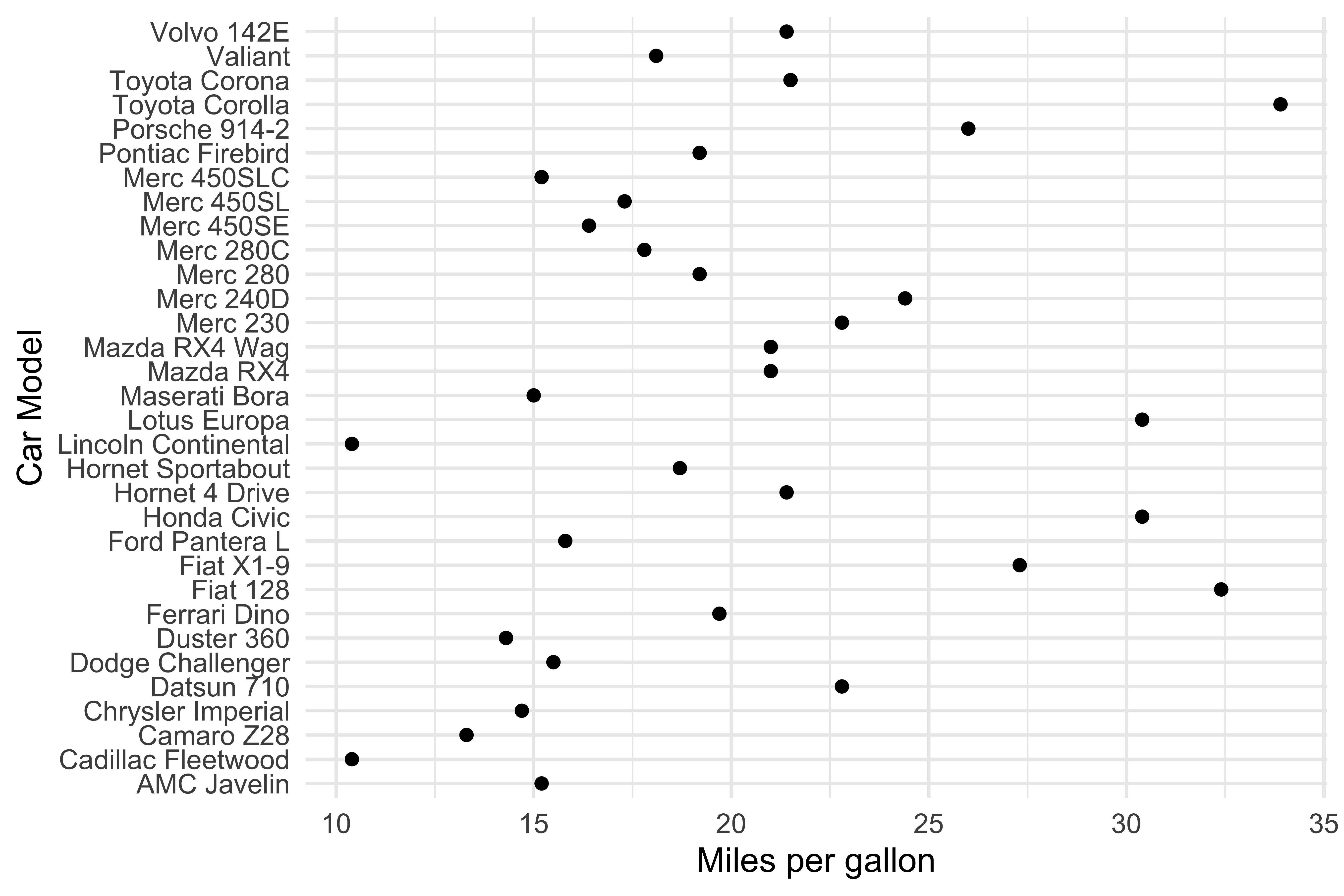
This isn't very helpful since the models are not arranged in ascending/descending order of miles per gallon. That can be easily fixed:
If I want the plot to be in descending order of mpg,
ggplot(mtcars, aes(x = mpg, fct_reorder(.f = model, .x = mpg))) + geom_point() + labs(x = "Miles per gallon", y = "Car Model") + theme_minimal()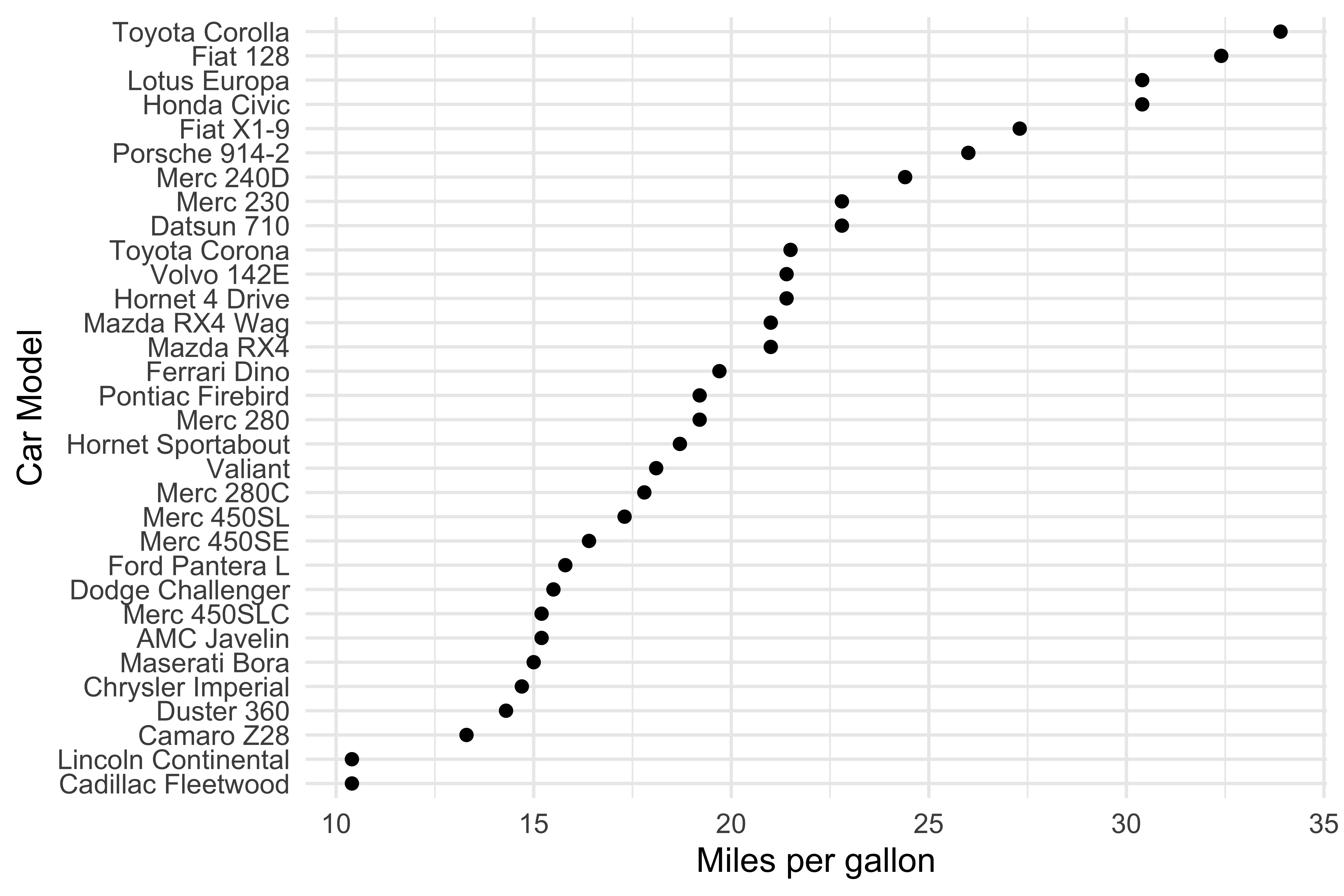
If I want the plot to be in descending order of mpg,
ggplot(mtcars, aes(x = mpg, fct_reorder(.f = model, .x = -mpg))) + geom_point() + labs(x = "Miles per gallon", y = "Car Model") + theme_minimal()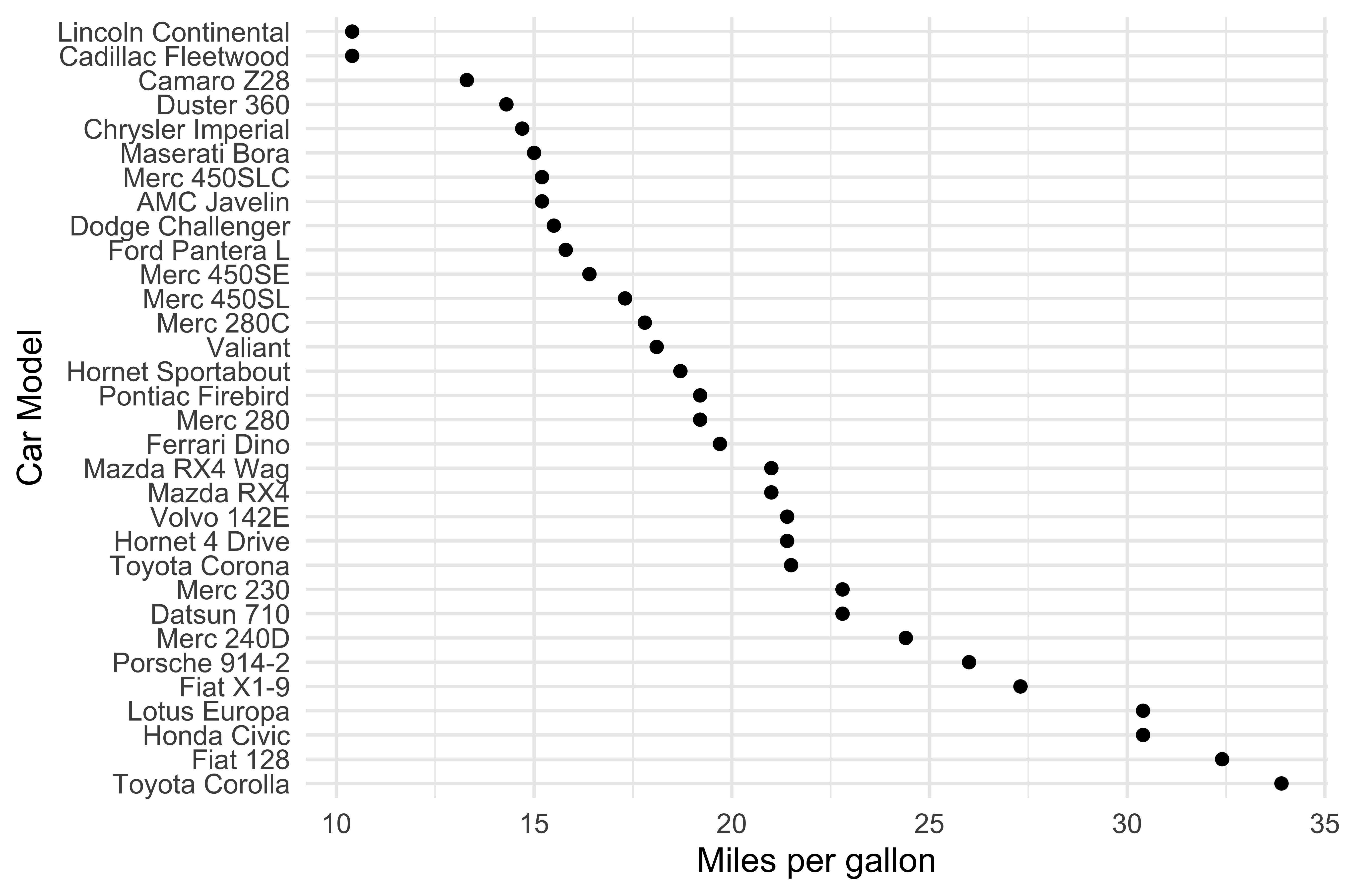
Note the use of .f and .x rather tha f and x
I can do this with bar-plots too.
ggplot(mtcars, aes(f.cyl)) + geom_bar(aes(fill = f.cyl)) + theme_minimal() + theme(legend.position = "none") + labs(x = "Number of cylinders", y = "Frequency")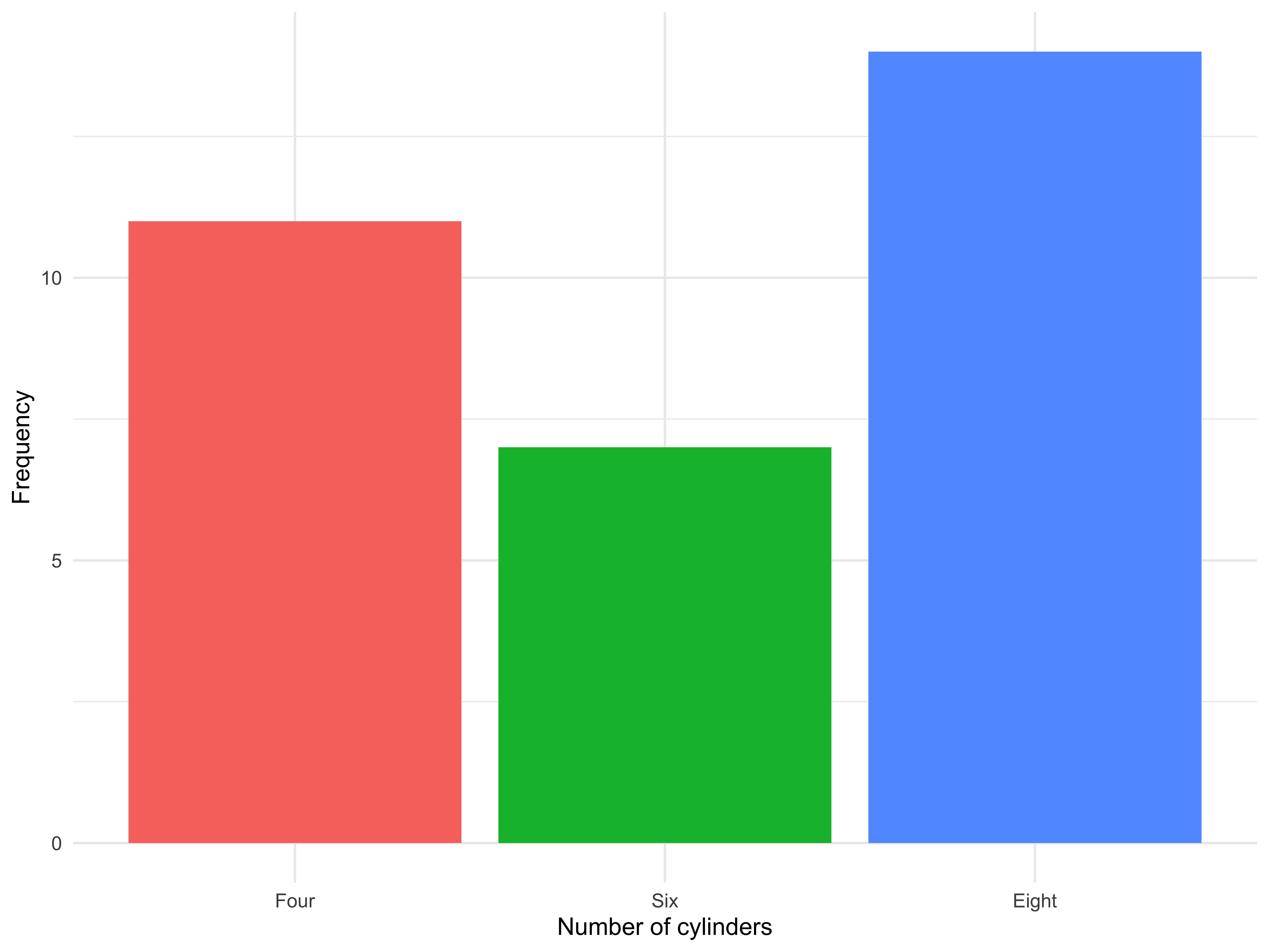
The bars ordered by descending frequency
ggplot(mtcars, aes(fct_infreq(f.cyl))) + geom_bar(aes(fill = f.cyl)) + theme_minimal() + theme(legend.position = "none") + labs(x = "Number of cylinders", y = "Frequency")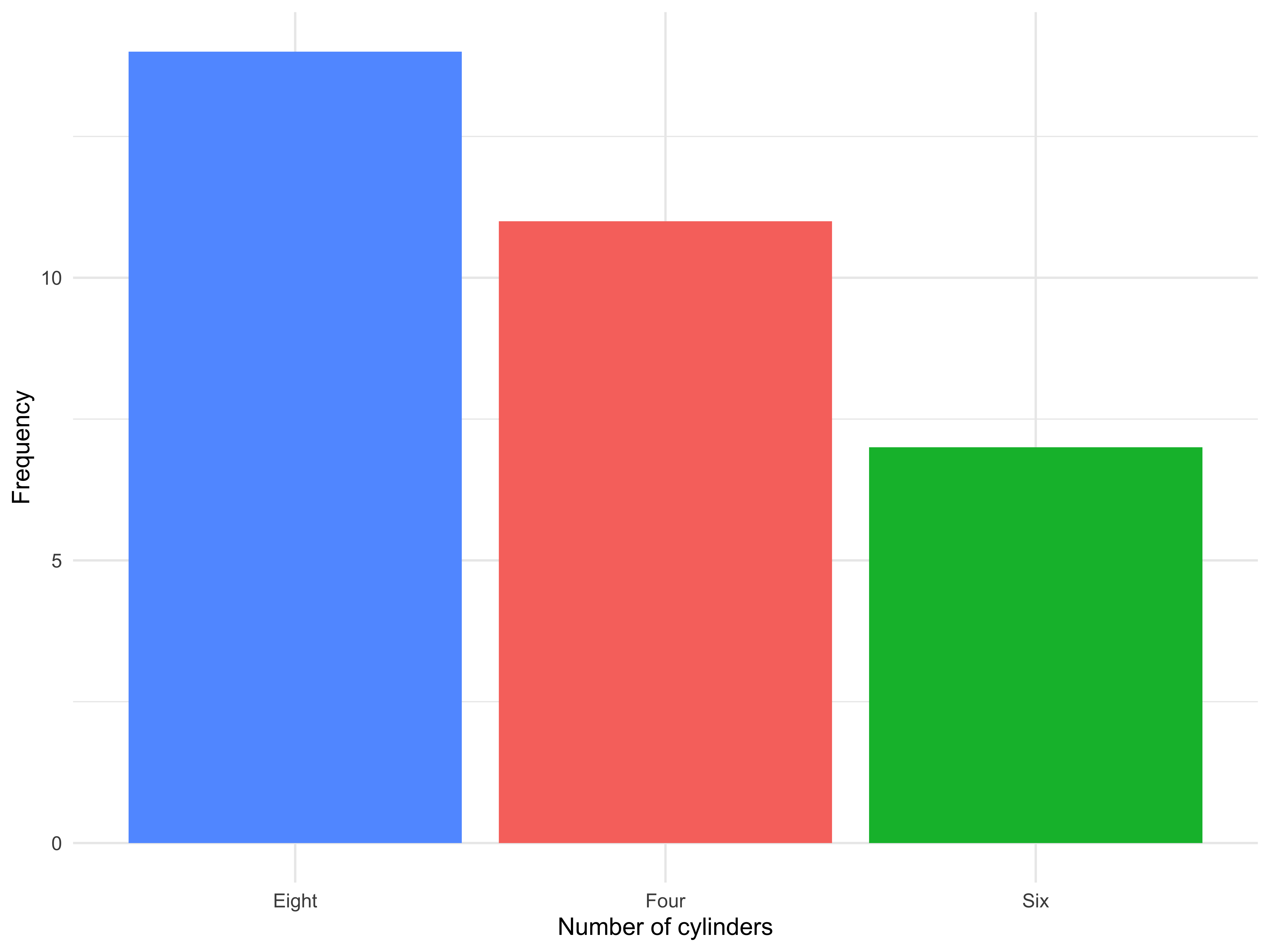
Note the use of fct_infreq() for descending
and the bars ordered by ascending frequency
ggplot(mtcars, aes(fct_rev(fct_infreq(f.cyl)))) + geom_bar(aes(fill = f.cyl)) + theme_minimal() + theme(legend.position = "none") + labs(x = "Number of cylinders", y = "Frequency")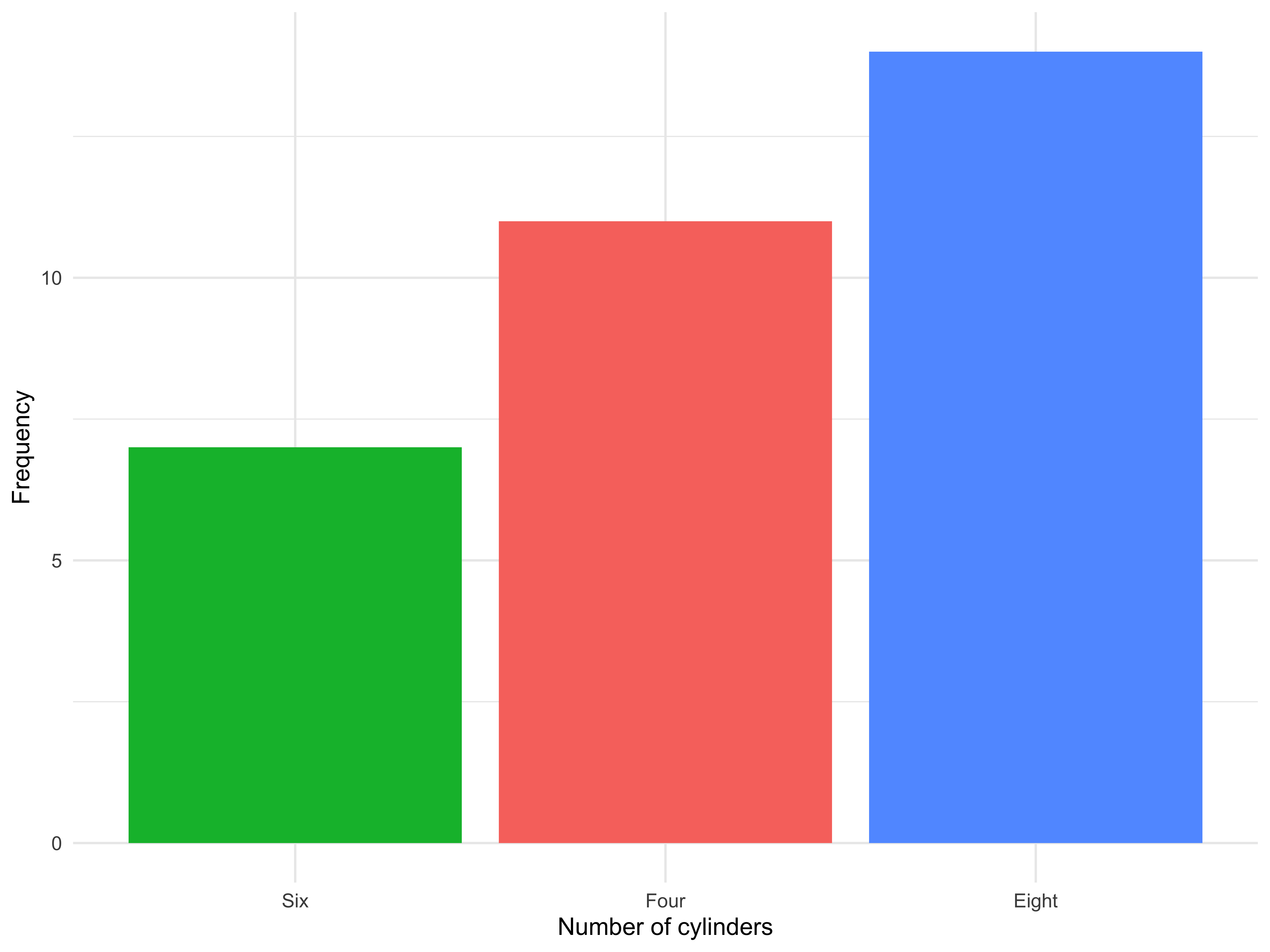
Note the use of fct_rev(fct_infreq()) for ascending.
Advanced dplyr
(or verbs I often forget exist in the dplyr stable)
select_if()
You can select columns based on logical and other criteria.
cmhflights2017 %>% select_if(is.character) %>% names()## [1] "Reporting_Airline" "IATA_CODE_Reporting_Airline"## [3] "Tail_Number" "Origin" ## [5] "OriginCityName" "OriginState" ## [7] "OriginStateFips" "OriginStateName" ## [9] "Dest" "DestCityName" ## [11] "DestState" "DestStateFips" ## [13] "DestStateName" "CRSDepTime" ## [15] "DepTime" "DepTimeBlk" ## [17] "WheelsOff" "WheelsOn" ## [19] "CRSArrTime" "ArrTime" ## [21] "ArrTimeBlk" "CancellationCode" ## [23] "FirstDepTime" "Div1Airport" ## [25] "Div1WheelsOn" "Div1WheelsOff" ## [27] "Div1TailNum"library(lubridate)cmhflights2017 %>% select_if(is.Date) %>% names()## [1] "FlightDate"cmhflights2017 %>% select_if(~is.numeric(.) & mean(., na.rm = TRUE) > 10 ) %>% names()## [1] "Year" "DayofMonth" ## [3] "DOT_ID_Reporting_Airline" "Flight_Number_Reporting_Airline"## [5] "OriginAirportID" "OriginAirportSeqID" ## [7] "OriginCityMarketID" "OriginWac" ## [9] "DestAirportID" "DestAirportSeqID" ## [11] "DestCityMarketID" "DestWac" ## [13] "DepDelayMinutes" "TaxiOut" ## [15] "ArrDelayMinutes" "CRSElapsedTime" ## [17] "ActualElapsedTime" "AirTime" ## [19] "Distance" "CarrierDelay" ## [21] "NASDelay" "LateAircraftDelay" ## [23] "TotalAddGTime" "LongestAddGTime" ## [25] "DivActualElapsedTime" "DivArrDelay" ## [27] "DivDistance" "Div1AirportID" ## [29] "Div1AirportSeqID" "Div1TotalGTime" ## [31] "Div1LongestGTime"You can also select with other conditions, for example, if the column has fewer than some number of distinct values ...
cmhflights2017 %>% select_if(~n_distinct(.) < 5) %>% names()## [1] "Year" "Quarter" "DepDel15" ## [4] "ArrDel15" "Cancelled" "CancellationCode" ## [7] "Diverted" "Flights" "DivAirportLandings"## [10] "DivReachedDest" "Div2Airport" "Div2AirportID" ## [13] "Div2AirportSeqID" "Div2WheelsOn" "Div2TotalGTime" ## [16] "Div2LongestGTime" "Div2WheelsOff" "Div2TailNum" ## [19] "Div3Airport" "Div3AirportID" "Div3AirportSeqID" ## [22] "Div3WheelsOn" "Div3TotalGTime" "Div3LongestGTime" ## [25] "Div3WheelsOff" "Div3TailNum" "Div4Airport" ## [28] "Div4AirportID" "Div4AirportSeqID" "Div4WheelsOn" ## [31] "Div4TotalGTime" "Div4LongestGTime" "Div4WheelsOff" ## [34] "Div4TailNum" "Div5Airport" "Div5AirportID" ## [37] "Div5AirportSeqID" "Div5WheelsOn" "Div5TotalGTime" ## [40] "Div5LongestGTime" "Div5WheelsOff" "Div5TailNum" ## [43] "X110"You can rearrange colums more swiftly too, as shown below where the first two columns I want are explicitly specified and then all remaining columns via everything()
df.ev <- cmhflights2017 %>% select(FlightDate, Flight_Number_Reporting_Airline, everything() )head(df.ev[, c(1:6)], 15)## FlightDate Flight_Number_Reporting_Airline id Year Quarter Month## 1 2017-01-02 2419 1 2017 1 1## 2 2017-01-02 2583 1 2017 1 1## 3 2017-01-03 977 1 2017 1 1## 4 2017-01-03 977 1 2017 1 1## 5 2017-01-03 1119 1 2017 1 1## 6 2017-01-03 1170 1 2017 1 1## 7 2017-01-03 1276 1 2017 1 1## 8 2017-01-03 1276 1 2017 1 1## 9 2017-01-03 1327 1 2017 1 1## 10 2017-01-03 1405 1 2017 1 1## 11 2017-01-03 1405 1 2017 1 1## 12 2017-01-03 1533 1 2017 1 1## 13 2017-01-03 1533 1 2017 1 1## 14 2017-01-03 1736 1 2017 1 1## 15 2017-01-03 1897 1 2017 1 1select_all
This is a very handy function as well since you can make sweeping changes very easily
cmhflights2017 %>% select_all(tolower) -> df.low names(df.low[, 1:10])## [1] "id" "year" ## [3] "quarter" "month" ## [5] "dayofmonth" "dayofweek" ## [7] "flightdate" "reporting_airline" ## [9] "dot_id_reporting_airline" "iata_code_reporting_airline"cmhflights2017 %>% select_all(tolower) %>% select_all(~str_replace_all(., "_", "")) -> df.low names(df.low[, 1:10])## [1] "id" "year" ## [3] "quarter" "month" ## [5] "dayofmonth" "dayofweek" ## [7] "flightdate" "reportingairline" ## [9] "dotidreportingairline" "iatacodereportingairline"select_at
This allows you to operate on selected variables if they meet a specific criterion
mtcars %>% select_at(vars(contains("ar"), starts_with("c")), toupper) %>% head()## GEAR CARB CYL## Mazda RX4 4 4 6## Mazda RX4 Wag 4 4 6## Datsun 710 4 1 4## Hornet 4 Drive 3 1 6## Hornet Sportabout 3 2 8## Valiant 3 1 6rownames_to_column
Some data-sets will have labels for rownames, as in the case of mtcars ... notice the first column is actually the row names
head(mtcars[, c(1:4)])## mpg cyl disp hp## Mazda RX4 21.0 6 160 110## Mazda RX4 Wag 21.0 6 160 110## Datsun 710 22.8 4 108 93## Hornet 4 Drive 21.4 6 258 110## Hornet Sportabout 18.7 8 360 175## Valiant 18.1 6 225 105mtcars %>% rownames_to_column() %>% head(3)## rowname mpg cyl disp hp drat wt qsec vs am gear carb f.cyl## 1 Mazda RX4 21.0 6 160 110 3.90 2.620 16.46 0 1 4 4 Six## 2 Mazda RX4 Wag 21.0 6 160 110 3.90 2.875 17.02 0 1 4 4 Six## 3 Datsun 710 22.8 4 108 93 3.85 2.320 18.61 1 1 4 1 Four## model## 1 Mazda RX4## 2 Mazda RX4 Wag## 3 Datsun 710mutate_at
This will allow you to mutate specific columns when the condition is met
mtcars %>% mutate_at(vars(contains("el")), tolower ) -> mut.df head(mut.df)## mpg cyl disp hp drat wt qsec vs am gear carb f.cyl## Mazda RX4 21.0 6 160 110 3.90 2.620 16.46 0 1 4 4 Six## Mazda RX4 Wag 21.0 6 160 110 3.90 2.875 17.02 0 1 4 4 Six## Datsun 710 22.8 4 108 93 3.85 2.320 18.61 1 1 4 1 Four## Hornet 4 Drive 21.4 6 258 110 3.08 3.215 19.44 1 0 3 1 Six## Hornet Sportabout 18.7 8 360 175 3.15 3.440 17.02 0 0 3 2 Eight## Valiant 18.1 6 225 105 2.76 3.460 20.22 1 0 3 1 Six## model## Mazda RX4 mazda rx4## Mazda RX4 Wag mazda rx4 wag## Datsun 710 datsun 710## Hornet 4 Drive hornet 4 drive## Hornet Sportabout hornet sportabout## Valiant valiantmtcars %>% mutate_at(vars(contains("pg")), ~(./10) ) -> mut.df head(mut.df)## mpg cyl disp hp drat wt qsec vs am gear carb f.cyl## Mazda RX4 2.10 6 160 110 3.90 2.620 16.46 0 1 4 4 Six## Mazda RX4 Wag 2.10 6 160 110 3.90 2.875 17.02 0 1 4 4 Six## Datsun 710 2.28 4 108 93 3.85 2.320 18.61 1 1 4 1 Four## Hornet 4 Drive 2.14 6 258 110 3.08 3.215 19.44 1 0 3 1 Six## Hornet Sportabout 1.87 8 360 175 3.15 3.440 17.02 0 0 3 2 Eight## Valiant 1.81 6 225 105 2.76 3.460 20.22 1 0 3 1 Six## model## Mazda RX4 Mazda RX4## Mazda RX4 Wag Mazda RX4 Wag## Datsun 710 Datsun 710## Hornet 4 Drive Hornet 4 Drive## Hornet Sportabout Hornet Sportabout## Valiant Valiantmutate_if
This is asking that if a column name has the string vs, that column should be converted into a factor
mtcars %>% mutate_if(is.factor, toupper ) -> mut.df head(mut.df)## mpg cyl disp hp drat wt qsec vs am gear carb f.cyl## Mazda RX4 21.0 6 160 110 3.90 2.620 16.46 0 1 4 4 SIX## Mazda RX4 Wag 21.0 6 160 110 3.90 2.875 17.02 0 1 4 4 SIX## Datsun 710 22.8 4 108 93 3.85 2.320 18.61 1 1 4 1 FOUR## Hornet 4 Drive 21.4 6 258 110 3.08 3.215 19.44 1 0 3 1 SIX## Hornet Sportabout 18.7 8 360 175 3.15 3.440 17.02 0 0 3 2 EIGHT## Valiant 18.1 6 225 105 2.76 3.460 20.22 1 0 3 1 SIX## model## Mazda RX4 Mazda RX4## Mazda RX4 Wag Mazda RX4 Wag## Datsun 710 Datsun 710## Hornet 4 Drive Hornet 4 Drive## Hornet Sportabout Hornet Sportabout## Valiant Valiantna_if
Here we are asking that if any variable mpg through vs has the value of 110, this value should be converted to NA (a missing value) ... compare values of hp across the left-right blocks of output
mtcars %>% select(mpg:vs) %>% na_if(110) -> naif.df head(naif.df)## mpg cyl disp hp drat wt qsec vs## Mazda RX4 21.0 6 160 NA 3.90 2.620 16.46 0## Mazda RX4 Wag 21.0 6 160 NA 3.90 2.875 17.02 0## Datsun 710 22.8 4 108 93 3.85 2.320 18.61 1## Hornet 4 Drive 21.4 6 258 NA 3.08 3.215 19.44 1## Hornet Sportabout 18.7 8 360 175 3.15 3.440 17.02 0## Valiant 18.1 6 225 105 2.76 3.460 20.22 1mtcars %>% select(mpg:vs) -> nonaif.df head(nonaif.df)## mpg cyl disp hp drat wt qsec vs## Mazda RX4 21.0 6 160 110 3.90 2.620 16.46 0## Mazda RX4 Wag 21.0 6 160 110 3.90 2.875 17.02 0## Datsun 710 22.8 4 108 93 3.85 2.320 18.61 1## Hornet 4 Drive 21.4 6 258 110 3.08 3.215 19.44 1## Hornet Sportabout 18.7 8 360 175 3.15 3.440 17.02 0## Valiant 18.1 6 225 105 2.76 3.460 20.22 1rowwise
This comes in handy if you have to operate on two or more columns but want the calculation done for each row. Here the average of mpg + qsec is being calculated for each model
mtcars %>% rowwise() %>% mutate(average = mean(c(mpg, qsec))) -> row.dfhead(row.df[, c(1, 7, 14)])## # A tibble: 6 x 3## # Rowwise: ## mpg qsec average## <dbl> <dbl> <dbl>## 1 21 16.5 18.7## 2 21 17.0 19.0## 3 22.8 18.6 20.7## 4 21.4 19.4 20.4## 5 18.7 17.0 17.9## 6 18.1 20.2 19.2between
As the name suggests, this allows you to filter for values that fall between the specified range (here mpg of 21 to 24). These boundary values are included in the filtered results
mtcars %>% filter(between(mpg, 21, 24) ) -> between.df between.df## mpg cyl disp hp drat wt qsec vs am gear carb f.cyl## Mazda RX4 21.0 6 160.0 110 3.90 2.620 16.46 0 1 4 4 Six## Mazda RX4 Wag 21.0 6 160.0 110 3.90 2.875 17.02 0 1 4 4 Six## Datsun 710 22.8 4 108.0 93 3.85 2.320 18.61 1 1 4 1 Four## Hornet 4 Drive 21.4 6 258.0 110 3.08 3.215 19.44 1 0 3 1 Six## Merc 230 22.8 4 140.8 95 3.92 3.150 22.90 1 0 4 2 Four## Toyota Corona 21.5 4 120.1 97 3.70 2.465 20.01 1 0 3 1 Four## Volvo 142E 21.4 4 121.0 109 4.11 2.780 18.60 1 1 4 2 Four## model## Mazda RX4 Mazda RX4## Mazda RX4 Wag Mazda RX4 Wag## Datsun 710 Datsun 710## Hornet 4 Drive Hornet 4 Drive## Merc 230 Merc 230## Toyota Corona Toyota Corona## Volvo 142E Volvo 142Enear
This allows you to filter within a range of values, the range specified via tol. Here, for example, we are asking for any case where mpg is inside the ±0.5 range of mpg=21, i.e., 20.5<x<21.5
mtcars %>% filter(near(mpg, 21, tol = 0.5) ) -> near.df near.df## mpg cyl disp hp drat wt qsec vs am gear carb f.cyl## Mazda RX4 21.0 6 160 110 3.90 2.620 16.46 0 1 4 4 Six## Mazda RX4 Wag 21.0 6 160 110 3.90 2.875 17.02 0 1 4 4 Six## Hornet 4 Drive 21.4 6 258 110 3.08 3.215 19.44 1 0 3 1 Six## Volvo 142E 21.4 4 121 109 4.11 2.780 18.60 1 1 4 2 Four## model## Mazda RX4 Mazda RX4## Mazda RX4 Wag Mazda RX4 Wag## Hornet 4 Drive Hornet 4 Drive## Volvo 142E Volvo 142Emtcars %>% filter(near(mpg, 21, tol = 0.5 * sd(mpg)) ) -> near.df head(near.df)## mpg cyl disp hp drat wt qsec vs am gear carb f.cyl## Mazda RX4 21.0 6 160 110 3.90 2.620 16.46 0 1 4 4 Six## Mazda RX4 Wag 21.0 6 160 110 3.90 2.875 17.02 0 1 4 4 Six## Datsun 710 22.8 4 108 93 3.85 2.320 18.61 1 1 4 1 Four## Hornet 4 Drive 21.4 6 258 110 3.08 3.215 19.44 1 0 3 1 Six## Hornet Sportabout 18.7 8 360 175 3.15 3.440 17.02 0 0 3 2 Eight## Valiant 18.1 6 225 105 2.76 3.460 20.22 1 0 3 1 Six## model## Mazda RX4 Mazda RX4## Mazda RX4 Wag Mazda RX4 Wag## Datsun 710 Datsun 710## Hornet 4 Drive Hornet 4 Drive## Hornet Sportabout Hornet Sportabout## Valiant Valiantxor
This is just another way of saying filter if mpg < 22 | cyl < 6
mtcars %>% filter(xor(mpg < 22, cyl < 6)) -> xor.df head(xor.df)## mpg cyl disp hp drat wt qsec vs am gear carb f.cyl## Mazda RX4 21.0 6 160 110 3.90 2.620 16.46 0 1 4 4 Six## Mazda RX4 Wag 21.0 6 160 110 3.90 2.875 17.02 0 1 4 4 Six## Datsun 710 22.8 4 108 93 3.85 2.320 18.61 1 1 4 1 Four## Hornet 4 Drive 21.4 6 258 110 3.08 3.215 19.44 1 0 3 1 Six## Hornet Sportabout 18.7 8 360 175 3.15 3.440 17.02 0 0 3 2 Eight## Valiant 18.1 6 225 105 2.76 3.460 20.22 1 0 3 1 Six## model## Mazda RX4 Mazda RX4## Mazda RX4 Wag Mazda RX4 Wag## Datsun 710 Datsun 710## Hornet 4 Drive Hornet 4 Drive## Hornet Sportabout Hornet Sportabout## Valiant Valiantmtcars %>% filter(mpg < 22 | cyl < 6) -> nonxor.df head(nonxor.df)## mpg cyl disp hp drat wt qsec vs am gear carb f.cyl## Mazda RX4 21.0 6 160 110 3.90 2.620 16.46 0 1 4 4 Six## Mazda RX4 Wag 21.0 6 160 110 3.90 2.875 17.02 0 1 4 4 Six## Datsun 710 22.8 4 108 93 3.85 2.320 18.61 1 1 4 1 Four## Hornet 4 Drive 21.4 6 258 110 3.08 3.215 19.44 1 0 3 1 Six## Hornet Sportabout 18.7 8 360 175 3.15 3.440 17.02 0 0 3 2 Eight## Valiant 18.1 6 225 105 2.76 3.460 20.22 1 0 3 1 Six## model## Mazda RX4 Mazda RX4## Mazda RX4 Wag Mazda RX4 Wag## Datsun 710 Datsun 710## Hornet 4 Drive Hornet 4 Drive## Hornet Sportabout Hornet Sportabout## Valiant Valiantfilter_all
This will filter all columns based on the condition specified, for example, findig all instances where baby names include the string "nnie"
library(babynames)babynames %>% filter_all(any_vars(str_detect(., pattern = "nnie")) ) -> filt.df head(filt.df)## # A tibble: 6 x 5## year sex name n prop## <dbl> <chr> <chr> <int> <dbl>## 1 1880 F Minnie 1746 0.0179 ## 2 1880 F Annie 1258 0.0129 ## 3 1880 F Jennie 793 0.00812 ## 4 1880 F Fannie 560 0.00574 ## 5 1880 F Nannie 248 0.00254 ## 6 1880 F Winnie 49 0.000502babynames %>% select_if(is.numeric) %>% filter_all(any_vars(. == 1880) ) -> filt.df head(filt.df)## # A tibble: 6 x 3## year n prop## <dbl> <int> <dbl>## 1 1880 7065 0.0724## 2 1880 2604 0.0267## 3 1880 2003 0.0205## 4 1880 1939 0.0199## 5 1880 1746 0.0179## 6 1880 1578 0.0162This has retained only those rows where at least one column/variable has a value of 1800
filter_if
This will allow you to filter if the logical condition is met, here if the column is a character column and if any character column has a missing value
starwars %>% filter_if(is.character, any_vars(is.na(.)) ) -> filt.df head(filt.df)## # A tibble: 6 x 14## name height mass hair_color skin_color eye_color birth_year sex gender## <chr> <int> <dbl> <chr> <chr> <chr> <dbl> <chr> <chr> ## 1 C-3PO 167 75 <NA> gold yellow 112 none mascu…## 2 R2-D2 96 32 <NA> white, blue red 33 none mascu…## 3 R5-D4 97 32 <NA> white, red red NA none mascu…## 4 Greedo 173 74 <NA> green black 44 male mascu…## 5 Jabba … 175 1358 <NA> green-tan,… orange 600 herma… mascu…## 6 Yoda 66 17 white green brown 896 male mascu…## # … with 5 more variables: homeworld <chr>, species <chr>, films <list>,## # vehicles <list>, starships <list>filter_at
This will come in very handy if you want to filter specific variables if a condition is met
mtcars %>% filter_at(vars(mpg, qsec), all_vars(. > 19) ) -> filt.df head(filt.df)## mpg cyl disp hp drat wt qsec vs am gear carb f.cyl## Hornet 4 Drive 21.4 6 258.0 110 3.08 3.215 19.44 1 0 3 1 Six## Merc 240D 24.4 4 146.7 62 3.69 3.190 20.00 1 0 4 2 Four## Merc 230 22.8 4 140.8 95 3.92 3.150 22.90 1 0 4 2 Four## Fiat 128 32.4 4 78.7 66 4.08 2.200 19.47 1 1 4 1 Four## Toyota Corolla 33.9 4 71.1 65 4.22 1.835 19.90 1 1 4 1 Four## Toyota Corona 21.5 4 120.1 97 3.70 2.465 20.01 1 0 3 1 Four## model## Hornet 4 Drive Hornet 4 Drive## Merc 240D Merc 240D## Merc 230 Merc 230## Fiat 128 Fiat 128## Toyota Corolla Toyota Corolla## Toyota Corona Toyota CoronaThis looked for mpg and qsec and then retained rows where either variable had a value > 19
mtcars %>% filter_at(vars(contains("t")), any_vars(. > 3) ) -> filt.df head(filt.df)## mpg cyl disp hp drat wt qsec vs am gear carb f.cyl## Mazda RX4 21.0 6 160 110 3.90 2.620 16.46 0 1 4 4 Six## Mazda RX4 Wag 21.0 6 160 110 3.90 2.875 17.02 0 1 4 4 Six## Datsun 710 22.8 4 108 93 3.85 2.320 18.61 1 1 4 1 Four## Hornet 4 Drive 21.4 6 258 110 3.08 3.215 19.44 1 0 3 1 Six## Hornet Sportabout 18.7 8 360 175 3.15 3.440 17.02 0 0 3 2 Eight## Valiant 18.1 6 225 105 2.76 3.460 20.22 1 0 3 1 Six## model## Mazda RX4 Mazda RX4## Mazda RX4 Wag Mazda RX4 Wag## Datsun 710 Datsun 710## Hornet 4 Drive Hornet 4 Drive## Hornet Sportabout Hornet Sportabout## Valiant ValiantHere we asked for columns with the letter t in their name, and any of these selected columns with values > 3
mtcars %>% filter_at(vars(contains("t")), all_vars(. > 3) ) -> filt.df head(filt.df)## mpg cyl disp hp drat wt qsec vs am gear carb f.cyl## Hornet 4 Drive 21.4 6 258.0 110 3.08 3.215 19.44 1 0 3 1 Six## Hornet Sportabout 18.7 8 360.0 175 3.15 3.440 17.02 0 0 3 2 Eight## Duster 360 14.3 8 360.0 245 3.21 3.570 15.84 0 0 3 4 Eight## Merc 240D 24.4 4 146.7 62 3.69 3.190 20.00 1 0 4 2 Four## Merc 230 22.8 4 140.8 95 3.92 3.150 22.90 1 0 4 2 Four## Merc 280 19.2 6 167.6 123 3.92 3.440 18.30 1 0 4 4 Six## model## Hornet 4 Drive Hornet 4 Drive## Hornet Sportabout Hornet Sportabout## Duster 360 Duster 360## Merc 240D Merc 240D## Merc 230 Merc 230## Merc 280 Merc 280Here we asked for columns with the letter t in their name, and all of these selected columns should have values > 3
summarise_all
Here we are asking that means be calculated for all selected variables -- mpg:qsec -- each on its own, of course
mtcars %>% select(mpg:qsec) %>% summarise_all(mean, na.rm = TRUE) -> summ.df summ.df## mpg cyl disp hp drat wt qsec## 1 20.09062 6.1875 230.7219 146.6875 3.596563 3.21725 17.84875summarise_if
Here we are asking for the means of specific variables -- if they are numeric -- to be calculated
mtcars %>% summarise_if(is.numeric, mean, na.rm = TRUE) %>% rename_if(is.numeric, ~paste0("mean_", .)) -> summ.df summ.df## mean_mpg mean_cyl mean_disp mean_hp mean_drat mean_wt mean_qsec mean_vs## 1 20.09062 6.1875 230.7219 146.6875 3.596563 3.21725 17.84875 0.4375## mean_am mean_gear mean_carb## 1 0.40625 3.6875 2.8125rename_if() is being used to append recognizable labels to the calculated values
summarise_at
Here we are asking for the means of specific variables -- those with the word "Delay" in their name -- to be calculated
cmhflights2017 %>% summarise_at(vars(contains("Delay")), mean, na.rm = TRUE) %>% rename_at(vars(contains("Delay")), ~paste0("mean_", .)) -> summ.df summ.df## mean_DepDelay mean_DepDelayMinutes mean_DepartureDelayGroups mean_ArrDelay## 1 8.756439 11.54685 -0.03739762 2.601107## mean_ArrDelayMinutes mean_ArrivalDelayGroups mean_CarrierDelay## 1 11.07277 -0.3285672 18.72072## mean_WeatherDelay mean_NASDelay mean_SecurityDelay mean_LateAircraftDelay## 1 2.676069 12.33165 0.04338477 26.01961## mean_DivArrDelay## 1 178.8784rename_at() is being used to append recognizable labels to the calculated values
top_n
This will give you the top or bottom n values (here n has been set to 7)
cmhflights2017 %>% group_by(Reporting_Airline) %>% filter(Dest == "CMH") %>% summarise(average.delay = mean(ArrDelay, na.rm = TRUE)) %>% arrange(-average.delay) %>% top_n(7)## # A tibble: 7 x 2## Reporting_Airline average.delay## <chr> <dbl>## 1 F9 7.54 ## 2 WN 5.20 ## 3 AA 4.92 ## 4 OO 4.66 ## 5 EV 0.966## 6 DL -1.01 ## 7 UA -2.27cmhflights2017 %>% group_by(Reporting_Airline) %>% filter(Dest == "CMH") %>% summarise(average.delay = mean(ArrDelay, na.rm = TRUE)) %>% arrange(average.delay) %>% top_n(-7)## # A tibble: 7 x 2## Reporting_Airline average.delay## <chr> <dbl>## 1 UA -2.27 ## 2 DL -1.01 ## 3 EV 0.966## 4 OO 4.66 ## 5 AA 4.92 ## 6 WN 5.20 ## 7 F9 7.54If you need to separate values accidentally stored in a single column into rows, use separate_rows
library(tibble)tibble( x = 1:3, y = c("a", "d,e,f", "g,h"), z = c("1", "2,3,4", "5,6") ) -> df df## # A tibble: 3 x 3## x y z ## <int> <chr> <chr>## 1 1 a 1 ## 2 2 d,e,f 2,3,4## 3 3 g,h 5,6separate_rows(df, y, z, convert = TRUE)## # A tibble: 6 x 3## x y z## <int> <chr> <int>## 1 1 a 1## 2 2 d 2## 3 2 e 3## 4 2 f 4## 5 3 g 5## 6 3 h 6dplyr's join
dplyr's join alternative to merge
dplyr has it own commands that execute what merge() did for us in the previous module. Let us see how this alternative route works but first we recreate the data we used with merge.
data.frame( Score = c(10, 21, 33, 12, 35, 67, 43, 99), ID = c("A12", "A23", "Z14", "WX1", "Y31", "D66", "C31", "Q22") ) -> data1 data.frame( Sex = c("Male", "Female", "Male", "Female", "Male", "Female", "Male", "Female"), ID = c("A12", "A23", "Z14", "WX1", "Y31", "D66", "E52", "H71") ) -> data2inner_join
This merges based on columns that appear in both data-sets, and will only merge rows that have the same value per column. In brief, only those observations common to both data-sets are retained.
inner_join(data1, data2, by = "ID")## Score ID Sex## 1 10 A12 Male## 2 21 A23 Female## 3 33 Z14 Male## 4 12 WX1 Female## 5 35 Y31 Male## 6 67 D66 FemaleIf you do not specify the by = column dplyr defaults to all columns with similar names in each data-set ...
inner_join(data1, data2)## Score ID Sex## 1 10 A12 Male## 2 21 A23 Female## 3 33 Z14 Male## 4 12 WX1 Female## 5 35 Y31 Male## 6 67 D66 Femaleleft_join
This merge will result in all rows being retained from the first data-set listed in the command, but will include only those rows from the second data-set that have the same value(s) for the by variable(s) ...
data1 %>% left_join(data2, by = "ID")## Score ID Sex## 1 10 A12 Male## 2 21 A23 Female## 3 33 Z14 Male## 4 12 WX1 Female## 5 35 Y31 Male## 6 67 D66 Female## 7 43 C31 <NA>## 8 99 Q22 <NA>data2 %>% left_join(data1, by = "ID")## Sex ID Score## 1 Male A12 10## 2 Female A23 21## 3 Male Z14 33## 4 Female WX1 12## 5 Male Y31 35## 6 Female D66 67## 7 Male E52 NA## 8 Female H71 NAright_join
This merge will result in all rows being retained from the second data-set listed in the command, but will include only those rows from the first data-set that have the same value(s) for the by variable(s) ...
data1 %>% right_join(data2, by = "ID")## Score ID Sex## 1 10 A12 Male## 2 21 A23 Female## 3 33 Z14 Male## 4 12 WX1 Female## 5 35 Y31 Male## 6 67 D66 Female## 7 NA E52 Male## 8 NA H71 Femaledata2 %>% right_join(data1, by = "ID")## Sex ID Score## 1 Male A12 10## 2 Female A23 21## 3 Male Z14 33## 4 Female WX1 12## 5 Male Y31 35## 6 Female D66 67## 7 <NA> C31 43## 8 <NA> Q22 99full_join
This merge keeps all rows from each data-set, with those only found in onde data-set being given NA values as necessary.
data1 %>% full_join(data2, by = "ID")## Score ID Sex## 1 10 A12 Male## 2 21 A23 Female## 3 33 Z14 Male## 4 12 WX1 Female## 5 35 Y31 Male## 6 67 D66 Female## 7 43 C31 <NA>## 8 99 Q22 <NA>## 9 NA E52 Male## 10 NA H71 Femalesemi_join
What if you only want observations that match in both data-sets and only those columns found in one data-set but not in the other? Use a semi-join. In the examples below, you will notice that the column Sex is not included in the first result since it is only found in data2 but is there in the second example since data2 is guiding the semi-Join().
data.frame( Score = c(10, 21, 33, 12, 35, 67, 43, 99), ID = c("A12", "A23", "Z14", "WX1", "Y31", "D66", "C31", "Q22") ) -> data1 data.frame( Score = c(10, 21, 33, 12, 35, 67, NA, NA), Sex = c("Male", "Female", "Male", "Female", "Male", "Female", "Male", "Female"), ID = c("A12", "A23", "Z14", "WX1", "Y31", "D66", "E52", "H71") ) -> data2semi_join(data1, data2)## Score ID## 1 10 A12## 2 21 A23## 3 33 Z14## 4 12 WX1## 5 35 Y31## 6 67 D66semi_join(data2, data1, by = "ID")## Score Sex ID## 1 10 Male A12## 2 21 Female A23## 3 33 Male Z14## 4 12 Female WX1## 5 35 Male Y31## 6 67 Female D66anti_join
This will only retain records not found in the second data-set listed.
anti_join(data1, data2)## Score ID## 1 43 C31## 2 99 Q22anti_join(data2, data1)## Score Sex ID## 1 NA Male E52## 2 NA Female H71vectorized functions in dplyr
Vectorized functions within mutate/transmute
You can create new columns by executing vectorized functions that vectors of some length as the input and return vectors of the same length as the output. These functions are shown below.
tibble::tibble( id = c( rep("A", 3), rep("B", 4), rep("C", 1), rep("D", 4) ), x = c(seq(1, 10, by = 1), -1, -2), y = c(seq(11, 20, by = 1), -11, -12) ) -> a.dfa.df## # A tibble: 12 x 3## id x y## <chr> <dbl> <dbl>## 1 A 1 11## 2 A 2 12## 3 A 3 13## 4 B 4 14## 5 B 5 15## 6 B 6 16## 7 B 7 17## 8 C 8 18## 9 D 9 19## 10 D 10 20## 11 D -1 -11## 12 D -2 -12lag() versus lead()
To lag some value implies to assign to the current observation (i.e., row) the preceding value. Similarly, to lead implies to assign to the current observation (i.e., row) the value from a subsequent row. If I lead by 1, then I am assiging the value from the next row, lead by 2 then I am assigning the value from 2 rows ahead, and so on. Say I want to lag the values of x by 1, first regardless of id but then within each id.
a.df %>% mutate(x.lag = lag(x, 1))## # A tibble: 12 x 4## id x y x.lag## <chr> <dbl> <dbl> <dbl>## 1 A 1 11 NA## 2 A 2 12 1## 3 A 3 13 2## 4 B 4 14 3## 5 B 5 15 4## 6 B 6 16 5## 7 B 7 17 6## 8 C 8 18 7## 9 D 9 19 8## 10 D 10 20 9## 11 D -1 -11 10## 12 D -2 -12 -1a.df %>% group_by(id) %>% mutate(x.lag = lag(x, 1))## # A tibble: 12 x 4## # Groups: id [4]## id x y x.lag## <chr> <dbl> <dbl> <dbl>## 1 A 1 11 NA## 2 A 2 12 1## 3 A 3 13 2## 4 B 4 14 NA## 5 B 5 15 4## 6 B 6 16 5## 7 B 7 17 6## 8 C 8 18 NA## 9 D 9 19 NA## 10 D 10 20 9## 11 D -1 -11 10## 12 D -2 -12 -1Similarly, I can also lead by a specific "period"
a.df %>% mutate(x.lead = lead(x, 2))## # A tibble: 12 x 4## id x y x.lead## <chr> <dbl> <dbl> <dbl>## 1 A 1 11 3## 2 A 2 12 4## 3 A 3 13 5## 4 B 4 14 6## 5 B 5 15 7## 6 B 6 16 8## 7 B 7 17 9## 8 C 8 18 10## 9 D 9 19 -1## 10 D 10 20 -2## 11 D -1 -11 NA## 12 D -2 -12 NAa.df %>% group_by(id) %>% mutate(y.lead = lead(y, 1))## # A tibble: 12 x 4## # Groups: id [4]## id x y y.lead## <chr> <dbl> <dbl> <dbl>## 1 A 1 11 12## 2 A 2 12 13## 3 A 3 13 NA## 4 B 4 14 15## 5 B 5 15 16## 6 B 6 16 17## 7 B 7 17 NA## 8 C 8 18 NA## 9 D 9 19 20## 10 D 10 20 -11## 11 D -1 -11 -12## 12 D -2 -12 NAcumulative aggregates
We can also calculate various aggregates by cumulating over/across columns.
c in any row is the smallest value observed thus far
a.df %>% mutate(c = cummin(x))## # A tibble: 12 x 4## id x y c## <chr> <dbl> <dbl> <dbl>## 1 A 1 11 1## 2 A 2 12 1## 3 A 3 13 1## 4 B 4 14 1## 5 B 5 15 1## 6 B 6 16 1## 7 B 7 17 1## 8 C 8 18 1## 9 D 9 19 1## 10 D 10 20 1## 11 D -1 -11 -1## 12 D -2 -12 -2c in any row is the largest value observed thus far
a.df %>% mutate(c = cummax(x))## # A tibble: 12 x 4## id x y c## <chr> <dbl> <dbl> <dbl>## 1 A 1 11 1## 2 A 2 12 2## 3 A 3 13 3## 4 B 4 14 4## 5 B 5 15 5## 6 B 6 16 6## 7 B 7 17 7## 8 C 8 18 8## 9 D 9 19 9## 10 D 10 20 10## 11 D -1 -11 10## 12 D -2 -12 10c is the average of the current + preceding value(s)
a.df %>% mutate(c = cummean(x))## # A tibble: 12 x 4## id x y c## <chr> <dbl> <dbl> <dbl>## 1 A 1 11 1 ## 2 A 2 12 1.5 ## 3 A 3 13 2 ## 4 B 4 14 2.5 ## 5 B 5 15 3 ## 6 B 6 16 3.5 ## 7 B 7 17 4 ## 8 C 8 18 4.5 ## 9 D 9 19 5 ## 10 D 10 20 5.5 ## 11 D -1 -11 4.91## 12 D -2 -12 4.33c is the cumulative sum of the current + preceding value(s)
a.df %>% mutate(c = cumsum(x))## # A tibble: 12 x 4## id x y c## <chr> <dbl> <dbl> <dbl>## 1 A 1 11 1## 2 A 2 12 3## 3 A 3 13 6## 4 B 4 14 10## 5 B 5 15 15## 6 B 6 16 21## 7 B 7 17 28## 8 C 8 18 36## 9 D 9 19 45## 10 D 10 20 55## 11 D -1 -11 54## 12 D -2 -12 52c is the cumulative product of the current value of x and the preceding value of c
a.df %>% mutate(c = cumprod(x))## # A tibble: 12 x 4## id x y c## <chr> <dbl> <dbl> <dbl>## 1 A 1 11 1## 2 A 2 12 2## 3 A 3 13 6## 4 B 4 14 24## 5 B 5 15 120## 6 B 6 16 720## 7 B 7 17 5040## 8 C 8 18 40320## 9 D 9 19 362880## 10 D 10 20 3628800## 11 D -1 -11 -3628800## 12 D -2 -12 7257600Say we have information on bank balance we hold by date. If the balance is negative, then we have leaned on an overdraft. We can use cumany() and cumall() to extract rows once a condition is met.
df <- data.frame( date = as.Date("2020-01-01") + 0:6, balance = c(100, 50, 25, -25, -50, 30, 120))df## date balance## 1 2020-01-01 100## 2 2020-01-02 50## 3 2020-01-03 25## 4 2020-01-04 -25## 5 2020-01-05 -50## 6 2020-01-06 30## 7 2020-01-07 120Show me all rows starting with when the first overdraft occurs
df %>% filter( cumany(balance < 0) )## date balance## 1 2020-01-04 -25## 2 2020-01-05 -50## 3 2020-01-06 30## 4 2020-01-07 120show me all rows preceding the first overdraft
df %>% filter( cumall(!(balance < 0)) )## date balance## 1 2020-01-01 100## 2 2020-01-02 50## 3 2020-01-03 25ranking functions
cume_dist()
This function gives a cumulative proportion of all values of x less than or equal to the current value.
a.df %>% mutate(d = cume_dist(x))## # A tibble: 12 x 4## id x y d## <chr> <dbl> <dbl> <dbl>## 1 A 1 11 0.25 ## 2 A 2 12 0.333 ## 3 A 3 13 0.417 ## 4 B 4 14 0.5 ## 5 B 5 15 0.583 ## 6 B 6 16 0.667 ## 7 B 7 17 0.75 ## 8 C 8 18 0.833 ## 9 D 9 19 0.917 ## 10 D 10 20 1 ## 11 D -1 -11 0.167 ## 12 D -2 -12 0.0833Note that -2 is the smallest value so it is ranked first, and the proportion becomes d = (1/12) = 0.0833.
-1 is bigger than -2, hence ranked second. Now d = (2/12) = 0.167 because two observations have a value of x equal to -1 or less.
And so on ...
row_number()
Say we have multiple observations for some group and want to flag whether a specific observation is the first, second, third, etc. within the group.
a.df %>% group_by(id) %>% mutate(flag_row = row_number())## # A tibble: 12 x 4## # Groups: id [4]## id x y flag_row## <chr> <dbl> <dbl> <int>## 1 A 1 11 1## 2 A 2 12 2## 3 A 3 13 3## 4 B 4 14 1## 5 B 5 15 2## 6 B 6 16 3## 7 B 7 17 4## 8 C 8 18 1## 9 D 9 19 1## 10 D 10 20 2## 11 D -1 -11 3## 12 D -2 -12 4If you want to flag in ascending or descending order of some variable, than you can run the following and when you do, pay attention to what happens with D since the smallest value of x is flagged as the first observation and NOT the order in which x appears in the data-set.
a.df %>% group_by(id) %>% mutate(flag_row = row_number(x))## # A tibble: 12 x 4## # Groups: id [4]## id x y flag_row## <chr> <dbl> <dbl> <int>## 1 A 1 11 1## 2 A 2 12 2## 3 A 3 13 3## 4 B 4 14 1## 5 B 5 15 2## 6 B 6 16 3## 7 B 7 17 4## 8 C 8 18 1## 9 D 9 19 3## 10 D 10 20 4## 11 D -1 -11 2## 12 D -2 -12 1min_rank() and percent_rank()
This allows you to flag the minimum rank for an observation as a rank or as a proportion
a.df %>% mutate(min.rank = min_rank(x))## # A tibble: 12 x 4## id x y min.rank## <chr> <dbl> <dbl> <int>## 1 A 1 11 3## 2 A 2 12 4## 3 A 3 13 5## 4 B 4 14 6## 5 B 5 15 7## 6 B 6 16 8## 7 B 7 17 9## 8 C 8 18 10## 9 D 9 19 11## 10 D 10 20 12## 11 D -1 -11 2## 12 D -2 -12 1a.df %>% group_by(id) %>% mutate(min.rank = min_rank(x))## # A tibble: 12 x 4## # Groups: id [4]## id x y min.rank## <chr> <dbl> <dbl> <int>## 1 A 1 11 1## 2 A 2 12 2## 3 A 3 13 3## 4 B 4 14 1## 5 B 5 15 2## 6 B 6 16 3## 7 B 7 17 4## 8 C 8 18 1## 9 D 9 19 3## 10 D 10 20 4## 11 D -1 -11 2## 12 D -2 -12 1a.df %>% mutate(pct.rank = percent_rank(x))## # A tibble: 12 x 4## id x y pct.rank## <chr> <dbl> <dbl> <dbl>## 1 A 1 11 0.182 ## 2 A 2 12 0.273 ## 3 A 3 13 0.364 ## 4 B 4 14 0.455 ## 5 B 5 15 0.545 ## 6 B 6 16 0.636 ## 7 B 7 17 0.727 ## 8 C 8 18 0.818 ## 9 D 9 19 0.909 ## 10 D 10 20 1 ## 11 D -1 -11 0.0909## 12 D -2 -12 0a.df %>% group_by(id) %>% mutate(pct.rank = percent_rank(x))## # A tibble: 12 x 4## # Groups: id [4]## id x y pct.rank## <chr> <dbl> <dbl> <dbl>## 1 A 1 11 0 ## 2 A 2 12 0.5 ## 3 A 3 13 1 ## 4 B 4 14 0 ## 5 B 5 15 0.333## 6 B 6 16 0.667## 7 B 7 17 1 ## 8 C 8 18 NaN ## 9 D 9 19 0.667## 10 D 10 20 1 ## 11 D -1 -11 0.333## 12 D -2 -12 0